EffectiveAreaTable

class gammapy.irf.EffectiveAreaTable(energy_lo, energy_hi, data, meta=None)

Bases: object

Effective area table.

TODO: Document

Parameters:

energy_lo : Quantity

Lower bin edges of energy axis

energy_hi : Quantity

Upper bin edges of energy axis

data : Quantity

Effective area

Examples

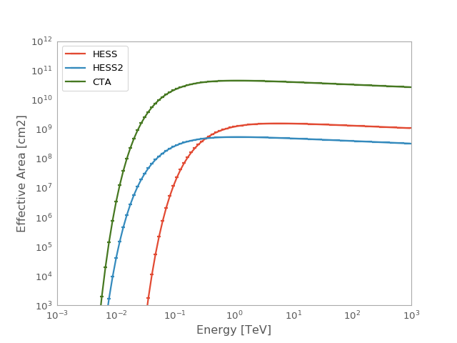
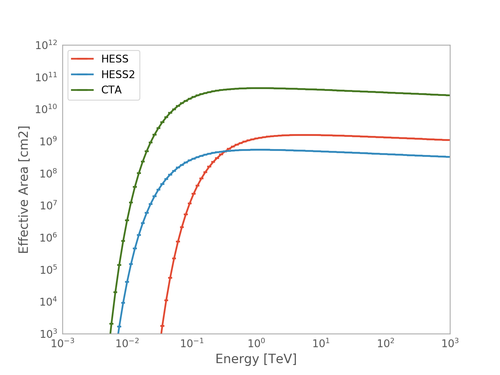
Plot parametrized effective area for HESS, HESS2 and CTA.

import numpy as np
import matplotlib.pyplot as plt
import astropy.units as u
from gammapy.irf import EffectiveAreaTable

energy = np.logspace(-3, 3, 100) * u.TeV

for instrument in ['HESS', 'HESS2', 'CTA']:
    aeff = EffectiveAreaTable.from_parametrization(energy, instrument)
    ax = aeff.plot(label=instrument)

ax.set_yscale('log')
ax.set_xlim([1e-3, 1e3])
ax.set_ylim([1e3, 1e12])
plt.legend(loc='best')
plt.show()

(Source code, png, hires.png, pdf)

Find energy where the effective area is at 10% of its maximum value

>>> import numpy as np
>>> from gammapy.irf import EffectiveAreaTable
>>> import astropy.units as u
>>> energy = np.logspace(-1,2) * u.TeV
>>> aeff_max = aeff.max_area
>>> print(aeff_max).to('m2')
156909.413371 m2
>>> ener = aeff.find_energy(0.1 * aeff_max)
>>> print(ener)
0.185368478744 TeV

Attributes Summary

energy
max_area	Maximum effective area

Methods Summary

evaluate_fill_nan(**kwargs)	Modified evaluate function.
find_energy(aeff)	Find energy for given effective area.
from_hdulist(hdulist[, hdu])
from_parametrization(energy[, instrument])	Get parametrized effective area.
from_table(table)	ARF reader
plot([ax, energy, show_energy])	Plot effective area.
read(filename[, hdu])
to_hdulist()
to_sherpa(name)	Return DataARF
to_table()	Convert to Table.
write(filename, **kwargs)

Attributes Documentation

energy

max_area

Maximum effective area

Methods Documentation

evaluate_fill_nan(**kwargs)

Modified evaluate function.

Calls gammapy.utils.nddata.NDDataArray.evaluate() and replaces possible nan values. Below the finite range the effective area is set to zero and above to value of the last valid note. This is needed since other codes, e.g. sherpa, don’t like nan values in FITS files. Make sure that the replacement happens outside of the energy range, where the EffectiveAreaTable is used.

find_energy(aeff)

Find energy for given effective area.

A linear interpolation is performed between the two nodes closest to the desired effective area value.

TODO: Move to NDDataArray

Parameters:

aeff : Quantity

Effective area value

Returns:

energy : Quantity

Energy corresponding to aeff

classmethod from_hdulist(hdulist, hdu='SPECRESP')

classmethod from_parametrization(energy, instrument='HESS')

Get parametrized effective area.

Parametrizations of the effective areas of different Cherenkov telescopes taken from Appendix B of Abramowski et al. (2010), see http://adsabs.harvard.edu/abs/2010MNRAS.402.1342A .

\[A_{eff}(E) = g_1 \left(\frac{E}{\mathrm{MeV}}\right)^{-g_2}\exp{\left(-\frac{g_3}{E}\right)}\]

Parameters:

energy : Quantity

Energy binning, analytic function is evaluated at log centers

instrument : {‘HESS’, ‘HESS2’, ‘CTA’}

Instrument name

classmethod from_table(table)

ARF reader

plot(ax=None, energy=None, show_energy=None, **kwargs)

Plot effective area.

Parameters:

ax : Axes, optional

Axis

energy : Quantity

Energy nodes

show_energy : Quantity, optional

Show energy, e.g. threshold, as vertical line

Returns:

ax : Axes

Axis

classmethod read(filename, hdu='SPECRESP', **kwargs)

to_hdulist()

to_sherpa(name)

Return DataARF

Parameters:

name : str

Instance name

to_table()

Convert to Table.

Data format specification: ARF file

write(filename, **kwargs)