Catalog & Simulation Images

The catalog_image method allows the production of single energy-band 2D images from point source catalogs, either true catalogs (e.g. 1FHL or 2FGL) or source catalogs of simulated galaxies (produced with population). Examples of these two use-cases are included below.

Source Catalog Images

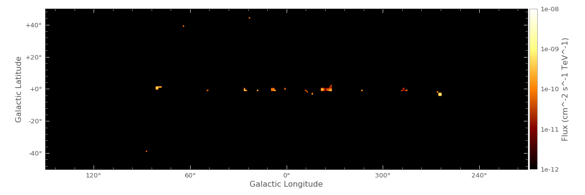
The example script below produces a point source catalog image from the published 1FHL Fermi Source Catalog from 10 to 500 GeV. Fluxes are filled into each pixel corresponding to source Galactic Latitude and Longitude, and then convolved with the Fermi PSF in this energy band.

"""Produces an image from 1FHL catalog point sources.
"""
import numpy as np
import matplotlib.pyplot as plt
from aplpy import FITSFigure
from gammapy.datasets import FermiGalacticCenter
from gammapy.image import catalog_image, SkyImage
from gammapy.irf import EnergyDependentTablePSF

# Create image of defined size
reference = SkyImage.empty(nxpix=300, nypix=100, binsz=1).to_image_hdu()
psf_file = FermiGalacticCenter.filenames()['psf']
psf = EnergyDependentTablePSF.read(psf_file)

# Create image
image = catalog_image(reference, psf, catalog='1FHL', source_type='point',
                      total_flux='True')

# Plot
fig = FITSFigure(image.to_fits(format='fermi-background')[0], figsize=(15, 5))
fig.show_colorscale(interpolation='bicubic', cmap='afmhot', stretch='log', vmin=1E-12, vmax=1E-8)
fig.tick_labels.set_xformat('ddd')
fig.tick_labels.set_yformat('dd')
ticks = np.logspace(-12, -8, 5)
fig.add_colorbar(ticks=ticks, axis_label_text='Flux (cm^-2 s^-1 TeV^-1)')
fig.colorbar._colorbar_axes.set_yticklabels(['{:.0e}'.format(_) for _ in ticks])
plt.tight_layout()
plt.show()

(Source code, png, hires.png, pdf)

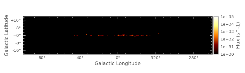
Simulated Catalog Images

In this case, a galaxy is simulated with population to produce a source catalog. This is then converted into an image.

"""Simulates a galaxy of point sources and produces an image.
"""
import numpy as np
import matplotlib.pyplot as plt
import astropy.units as u
from aplpy import FITSFigure
from gammapy.astro import population
from gammapy.datasets import FermiGalacticCenter
from gammapy.image import SkyImage, catalog_image
from gammapy.irf import EnergyDependentTablePSF
from gammapy.utils.random import sample_powerlaw

# Create image of defined size
reference = SkyImage.empty(nxpix=1000, nypix=200, binsz=0.2).to_image_hdu()

psf_file = FermiGalacticCenter.filenames()['psf']
psf = EnergyDependentTablePSF.read(psf_file)

# Simulation Parameters
n_sources = int(5e2)

table = population.make_base_catalog_galactic(
    n_sources=n_sources,
    rad_dis='L06',
    vel_dis='F06B',
    max_age=1e5 * u.yr,
    spiralarms=True,
    random_state=0,
)

# Minimum source luminosity (s^-1)
luminosity_min = 4e34
# Maximum source luminosity (s^-1)
luminosity_max = 4e37
# Luminosity function differential power-law index
luminosity_index = 1.5

# Assigns luminosities to sources
luminosity = sample_powerlaw(luminosity_min, luminosity_max, luminosity_index,
                             n_sources, random_state=0)
table['luminosity'] = luminosity

# Adds parameters to table: distance, glon, glat, flux, angular_extension
table = population.add_observed_parameters(table)
table.meta['Energy Bins'] = [10, 500] * u.GeV
# Create image
image = catalog_image(reference, psf, catalog='simulation', source_type='point',
                      total_flux=True, sim_table=table)

# Plot
fig = FITSFigure(image.to_fits(format='fermi-background')[0], figsize=(10, 3))
fig.show_colorscale(interpolation='bicubic', cmap='afmhot', stretch='log', vmin=1E30, vmax=1E35)
fig.tick_labels.set_xformat('ddd')
fig.tick_labels.set_yformat('dd')
ticks = np.logspace(30, 35, 6)
fig.add_colorbar(ticks=ticks, axis_label_text='Flux (s^-1)')
fig.colorbar._colorbar_axes.set_yticklabels(['{:.0e}'.format(_) for _ in ticks])
plt.tight_layout()
plt.show()

(Source code, png, hires.png, pdf)

Caveats & Future Developments

It should be noted that the current implementation does not support:

• The inclusion of extended sources
• Production of images in more than one energy band