Fermi-LAT diffuse model predicted counts image¶

The SkyCube class allows for image-based analysis in energy bands. In particular, similar functionality to gtmodel in the Fermi Science tools [FSSC2013] is offered in compute_npred_cube which generates a predicted instrument PSF-convolved counts cube based on a provided background model. Unlike the science tools, this implementation is appropriate for use with large regions of the sky.

Predicting Counts¶

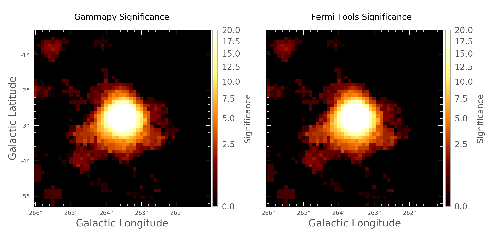
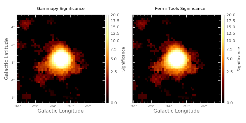
The example script below computes the Fermi PSF-convolved predicted counts map using SkyCube. This is then used to produce a Li & Ma significance image [LiMa1983]. The left image shows the significance image, while a comparison against the significance image produced using the Fermi Science tools is shown on the right. These results are for the Vela region for energies between 10 and 500 GeV.

"""Runs commands to produce convolved predicted counts map in current directory."""
import numpy as np
from astropy.coordinates import Angle
from astropy.units import Quantity
from astropy.io import fits
from astropy.wcs import WCS
from gammapy.cube import SkyCube, compute_npred_cube
from gammapy.datasets import FermiVelaRegion
from gammapy.irf import EnergyDependentTablePSF
from gammapy.utils.energy import EnergyBounds

__all__ = ['prepare_images']


def prepare_images():
    # Read in data
    fermi_vela = FermiVelaRegion()
    background_file = FermiVelaRegion.filenames()['diffuse_model']
    exposure_file = FermiVelaRegion.filenames()['exposure_cube']
    counts_file = FermiVelaRegion.filenames()['counts_cube']
    background_model = SkyCube.read(background_file, format='fermi-background')
    exposure_cube = SkyCube.read(exposure_file, format='fermi-exposure')

    # Re-project background cube
    repro_bg_cube = background_model.reproject(exposure_cube)

    # Define energy band required for output
    energies = EnergyBounds([10, 500], 'GeV')

    # Compute the predicted counts cube
    npred_cube = compute_npred_cube(repro_bg_cube, exposure_cube, energies,
                                    integral_resolution=5)

    # Convolve with Energy-dependent Fermi LAT PSF
    psf = EnergyDependentTablePSF.read(FermiVelaRegion.filenames()['psf'])
    kernels = psf.kernels(npred_cube)
    convolved_npred_cube = npred_cube.convolve(kernels, mode='reflect')

    # Counts data
    counts_cube = SkyCube.read(counts_file, format='fermi-counts')
    counts_cube = counts_cube.reproject(npred_cube)

    counts = counts_cube.data[0]
    model = convolved_npred_cube.data[0]

    # Load Fermi tools gtmodel background-only result
    gtmodel = fits.open(FermiVelaRegion.filenames()['background_image'])[0].data.astype(float)

    # Ratio for the two background images
    ratio = np.nan_to_num(model / gtmodel)

    # Header is required for plotting, so returned here
    wcs = npred_cube.wcs
    header = wcs.to_header()
    return model, gtmodel, ratio, counts, header

"""Runs commands to produce convolved predicted counts map in current directory."""
import numpy as np
import matplotlib.pyplot as plt
from astropy.io import fits
from astropy.convolution import Tophat2DKernel
from scipy.ndimage import convolve
from gammapy.stats import significance
from aplpy import FITSFigure
from npred_general import prepare_images

model, gtmodel, ratio, counts, header = prepare_images()

# Top hat correlation
tophat = Tophat2DKernel(3)
tophat.normalize('peak')

correlated_gtmodel = convolve(gtmodel, tophat.array)
correlated_counts = convolve(counts, tophat.array)
correlated_model = convolve(model, tophat.array)

# Fermi significance
fermi_significance = np.nan_to_num(significance(correlated_counts, correlated_gtmodel,
                                                method='lima'))
# Gammapy significance
significance = np.nan_to_num(significance(correlated_counts, correlated_model,
                                          method='lima'))

titles = ['Gammapy Significance', 'Fermi Tools Significance']

# Plot

fig = plt.figure(figsize=(10, 5))
hdu1 = fits.ImageHDU(significance, header)
f1 = FITSFigure(hdu1, figure=fig, convention='wells', subplot=(1, 2, 1))
f1.set_tick_labels_font(size='x-small')
f1.tick_labels.set_xformat('ddd')
f1.tick_labels.set_yformat('ddd')
f1.show_colorscale(vmin=0, vmax=20, cmap='afmhot', stretch='sqrt')
f1.add_colorbar(axis_label_text='Significance')
f1.colorbar.set_width(0.1)
f1.colorbar.set_location('right')

hdu2 = fits.ImageHDU(fermi_significance, header)
f2 = FITSFigure(hdu2, figure=fig, convention='wells', subplot=(1, 2, 2))
f2.set_tick_labels_font(size='x-small')
f2.tick_labels.set_xformat('ddd')
f2.hide_ytick_labels()
f2.hide_yaxis_label()
f2.show_colorscale(vmin=0, vmax=20, cmap='afmhot', stretch='sqrt')
f2.add_colorbar(axis_label_text='Significance')
f2.colorbar.set_width(0.1)
f2.colorbar.set_location('right')
fig.text(0.15, 0.92, "Gammapy Significance")
fig.text(0.63, 0.92, "Fermi Tools Significance")
plt.tight_layout()
plt.show()

(Source code, png, hires.png, pdf)

../../_images/npred_convolved_significance.png

Checks¶

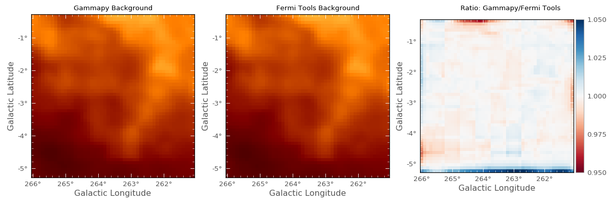
For small regions, the predicted counts cube and significance images may be checked against the gtmodel output. The Vela region shown above is taken in this example in one energy band with the parameters outlined in the README file for FermiVelaRegion.

Images for the predicted background counts in this region in the Gammapy case (left) and Fermi Science Tools gtmodel case (center) are shown below, based on the differential flux contribution of the Fermi diffuse model gll_iem_v05_rev1.fit. The image on the right shows the ratio. Note that the colorbar scale applies only to the ratio image.

"""Runs commands to produce convolved predicted counts map in current directory.
"""
import matplotlib.pyplot as plt
from astropy.io import fits
from aplpy import FITSFigure
from npred_general import prepare_images

model, gtmodel, ratio, counts, header = prepare_images()

# Plotting
fig = plt.figure(figsize=(15, 5))

image1 = fits.ImageHDU(data=model, header=header)
f1 = FITSFigure(image1, figure=fig, subplot=(1, 3, 1), convention='wells')
f1.show_colorscale(vmin=0, vmax=0.3, cmap='afmhot')
f1.tick_labels.set_xformat('ddd')
f1.tick_labels.set_yformat('dd')

image2 = fits.ImageHDU(data=gtmodel, header=header)
f2 = FITSFigure(image2, figure=fig, subplot=(1, 3, 2), convention='wells')
f2.show_colorscale(vmin=0, vmax=0.3, cmap='afmhot')
f2.tick_labels.set_xformat('ddd')
f2.tick_labels.set_yformat('dd')

image3 = fits.ImageHDU(data=ratio, header=header)
f3 = FITSFigure(image3, figure=fig, subplot=(1, 3, 3), convention='wells')
f3.show_colorscale(vmin=0.95, vmax=1.05, cmap='RdBu')
f3.tick_labels.set_xformat('ddd')
f3.tick_labels.set_yformat('dd')
f3.add_colorbar(ticks=[0.95, 0.975, 1, 1.025, 1.05])

fig.text(0.12, 0.95, "Gammapy Background")
fig.text(0.45, 0.95, "Fermi Tools Background")
fig.text(0.75, 0.95, "Ratio: Gammapy/Fermi Tools")
plt.tight_layout()
plt.show()

(Source code, png, hires.png, pdf)

We may compare these against the true counts observed by Fermi LAT in this region for the same parameters:

True total counts: 1551

Fermi Tools gtmodel predicted background counts: 265

Gammapy predicted background counts: 282

Navigation

Fermi-LAT diffuse model predicted counts image¶

Predicting Counts¶

Checks¶