This is a fixed-text formatted version of a Jupyter notebook.
You can contribute with your own notebooks in this GitHub repository.
Source files: cta_data_analysis.ipynb | cta_data_analysis.py

CTA first data challenge logo
CTA data analysis with Gammapy
Introduction
This notebook shows an example how to make a sky image and spectrum for simulated CTA data with Gammapy.
The dataset we will use is three observation runs on the Galactic center. This is a tiny (and thus quick to process and play with and learn) subset of the simulated CTA dataset that was produced for the first data challenge in August 2017.
This notebook can be considered part 2 of the introduction to CTA 1DC analysis. Part one is here: `cta_1dc_introduction.ipynb <cta_1dc_introduction.ipynb>`__
Setup
As usual, we’ll start with some setup …
In [1]:
%matplotlib inline
import matplotlib.pyplot as plt
In [2]:
# Check package versions, if something goes wrong here you won't be able to run the notebook
import gammapy
import numpy as np
import astropy
import regions
import sherpa
import uncertainties
import photutils

print('gammapy:', gammapy.__version__)
print('numpy:', np.__version__)
print('astropy:', astropy.__version__)
print('regions:', regions.__version__)
print('sherpa:', sherpa.__version__)
print('uncertainties:', uncertainties.__version__)
print('photutils:', photutils.__version__)
gammapy: 0.7.dev5344
numpy: 1.13.3
astropy: 3.0.dev20763
regions: 0.2
sherpa: 4.9.1+12.g3626715
uncertainties: 2.4.8.1
photutils: 0.3.2
In [3]:
import numpy as np
import astropy.units as u
from astropy.coordinates import SkyCoord, Angle
from regions import CircleSkyRegion
from photutils.detection import find_peaks
from gammapy.data import DataStore
from gammapy.spectrum import (
    SpectrumExtraction,
    SpectrumFit,
    SpectrumResult,
    models,
    SpectrumEnergyGroupMaker,
    FluxPointEstimator,
)
from gammapy.image import SkyImage, IACTBasicImageEstimator
from gammapy.background import RingBackgroundEstimator, ReflectedRegionsBackgroundEstimator
from gammapy.utils.energy import EnergyBounds
from gammapy.detect import TSImageEstimator
In [4]:
# Configure the logger, so that the spectral analysis
# isn't so chatty about what it's doing.
import logging
logging.basicConfig()
log = logging.getLogger('gammapy.spectrum')
log.setLevel(logging.ERROR)
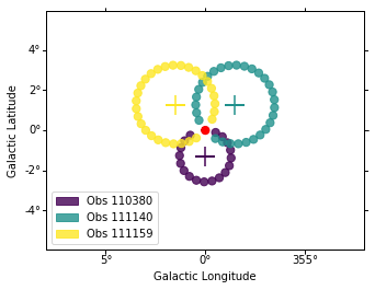
Select observations
Like explained in
cta_1dc_introduction.ipynb, a Gammapy
analysis usually starts by creating a DataStore and selecting
observations.
This is shown in detail in the other notebook, here we just pick three observations near the galactic center.
In [5]:
data_store = DataStore.from_dir('$CTADATA/index/gps')
In [6]:
# Just as a reminder: this is how to select observations
# from astropy.coordinates import SkyCoord
# table = data_store.obs_table
# pos_obs = SkyCoord(table['GLON_PNT'], table['GLAT_PNT'], frame='galactic', unit='deg')
# pos_target = SkyCoord(0, 0, frame='galactic', unit='deg')
# offset = pos_target.separation(pos_obs).deg
# mask = (1 < offset) & (offset < 2)
# table = table[mask]
# table.show_in_browser(jsviewer=True)
In [7]:
obs_id = [110380, 111140, 111159]
obs_list = data_store.obs_list(obs_id)
In [8]:
obs_cols = ['OBS_ID', 'GLON_PNT', 'GLAT_PNT', 'LIVETIME']
data_store.obs_table.select_obs_id(obs_id)[obs_cols]
Out[8]:
| OBS_ID | GLON_PNT | GLAT_PNT | LIVETIME |
|---|---|---|---|
| int64 | float64 | float64 | float64 |
| 110380 | 359.999991204 | -1.29999593791 | 1764.0 |
| 111140 | 358.499983383 | 1.3000020212 | 1764.0 |
| 111159 | 1.50000565683 | 1.29994046834 | 1764.0 |
Make sky images
Define map geometry
Select the target position and define an ON region for the spectral analysis
In [9]:
target_position = SkyCoord(0, 0, unit='deg', frame='galactic')
on_radius = 0.2 * u.deg
on_region = CircleSkyRegion(center=target_position, radius=on_radius)
In [10]:
# Define reference image centered on the target
xref = target_position.galactic.l.value
yref = target_position.galactic.b.value
# size = 10 * u.deg
# binsz = 0.02 # degree per pixel
# npix = int((size / binsz).value)

ref_image = SkyImage.empty(
    nxpix=800, nypix=600, binsz=0.02,
    xref=xref, yref=yref,
    proj='TAN', coordsys='GAL',
)
print(ref_image)
Name: None
Data shape: (600, 800)
Data type: float64
Data unit:
Data mean: 0.000e+00
WCS type: ['GLON-TAN', 'GLAT-TAN']
Compute images
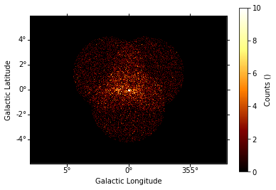
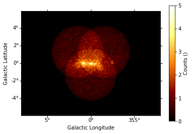
We use the ring background estimation method, and an exclusion mask that excludes the bright source at the Galactic center.
In [11]:
exclusion_mask = ref_image.region_mask(on_region)
exclusion_mask.data = 1 - exclusion_mask.data
exclusion_mask.plot()
Out[11]:
(<matplotlib.figure.Figure at 0x10443af98>,
 <matplotlib.axes._subplots.WCSAxesSubplot at 0x1094d8390>,
 None)
In [12]:
bkg_estimator = RingBackgroundEstimator(
    r_in=0.5 * u.deg,
    width=0.2 * u.deg,
)
image_estimator = IACTBasicImageEstimator(
    reference=ref_image,
    emin=100 * u.GeV,
    emax=100 * u.TeV,
    offset_max=3 * u.deg,
    background_estimator=bkg_estimator,
    exclusion_mask=exclusion_mask,
)
images = image_estimator.run(obs_list)
images.names
/Users/deil/code/gammapy/gammapy/cube/core.py:76: RuntimeWarning: divide by zero encountered in log
  log_data = np.log(self.data.value)
/opt/local/Library/Frameworks/Python.framework/Versions/3.6/lib/python3.6/site-packages/scipy/interpolate/interpolate.py:2477: RuntimeWarning: invalid value encountered in multiply
  values += np.asarray(self.values[edge_indices]) * weight[vslice]
WARNING: AstropyDeprecationWarning: The truth value of a Quantity is ambiguous. In the future this will raise a ValueError. [astropy.units.quantity]
WARNING:astropy:AstropyDeprecationWarning: The truth value of a Quantity is ambiguous. In the future this will raise a ValueError.
Out[12]:
['counts', 'exposure', 'background', 'excess', 'flux', 'psf']
Show images
Let’s define a little helper function and then show all the resulting images that were computed.
In [13]:
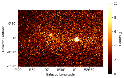
def show_image(image, radius=3, vmin=0, vmax=3):
    """Little helper function to show the images for this application here."""
    image.smooth(radius=radius).show(vmin=vmin, vmax=vmax, add_cbar=True)
    image.cutout(
        position=SkyCoord(0.5, 0, unit='deg', frame='galactic'),
        size=(2*u.deg, 3*u.deg),
    ).smooth(radius=radius).show(vmin=vmin, vmax=vmax, add_cbar=True)
In [14]:
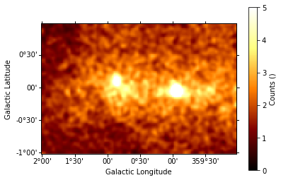
show_image(images['counts'], radius=0, vmax=10)
In [15]:
show_image(images['counts'], vmax=5)
In [16]:
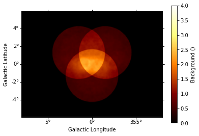
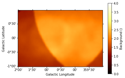
show_image(images['background'], vmax=4)
In [17]:
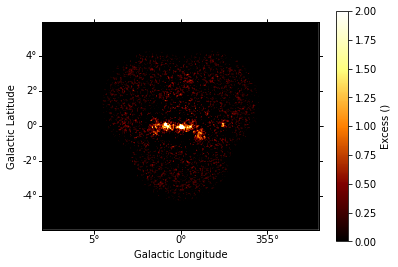
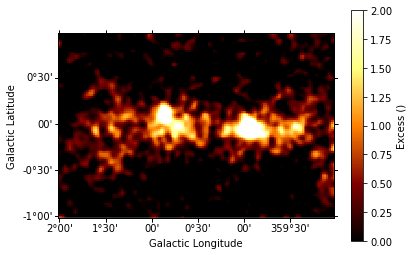
show_image(images['excess'], vmax=2)
In [18]:
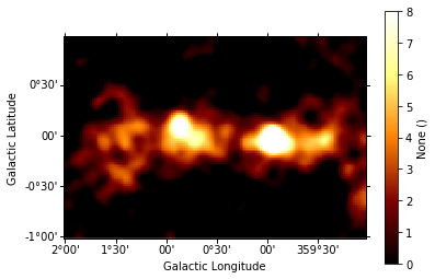
# Significance image
# Just for fun, let's compute it by hand ...
from astropy.convolution import Tophat2DKernel
kernel = Tophat2DKernel(4)
kernel.normalize('peak')

counts_conv = images['counts'].convolve(kernel.array)
background_conv = images['background'].convolve(kernel.array)

from gammapy.stats import significance
significance_image = SkyImage.empty_like(ref_image)
significance_image.data = significance(counts_conv.data, background_conv.data)
show_image(significance_image, vmax=8)
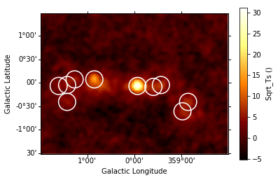
Source Detection
Use the class TSImageEstimator and photutils.find_peaks to detect point-like sources on the images:
In [19]:
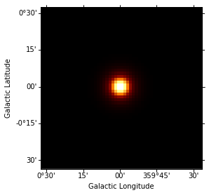
# cut out smaller piece of the PSF image to save computing time
# for covenience we're "misusing" the SkyImage class represent the PSF on the sky.
kernel = images['psf'].cutout(target_position, size= 1.1 * u.deg)
kernel.show()
In [20]:
ts_image_estimator = TSImageEstimator()
images_ts = ts_image_estimator.run(images, kernel.data)
print(images_ts.names)
['ts', 'sqrt_ts', 'flux', 'flux_err', 'flux_ul', 'niter']
In [21]:
# find pointlike sources with sqrt(TS) > 5
sources = find_peaks(data=images_ts['sqrt_ts'].data, threshold=5, wcs=images_ts['sqrt_ts'].wcs)
sources
/opt/local/Library/Frameworks/Python.framework/Versions/3.6/lib/python3.6/site-packages/photutils/detection/core.py:241: RuntimeWarning: invalid value encountered in greater
  peak_goodmask = np.logical_and(peak_goodmask, (data > threshold))
Out[21]:
| x_peak | y_peak | icrs_ra_peak | icrs_dec_peak | peak_value |
|---|---|---|---|---|
| deg | deg | |||
| int64 | int64 | float64 | float64 | float64 |
| 451 | 269 | 266.386490097 | -30.1329751991 | 6.43453671617 |
| 328 | 279 | 267.643982436 | -27.923799443 | 5.01020960141 |
| 457 | 279 | 266.116882008 | -30.1308815126 | 6.99895391199 |
| 420 | 295 | 266.248069224 | -29.332923145 | 7.40642882084 |
| 319 | 296 | 267.418588423 | -27.5950146565 | 5.43758078846 |
| 403 | 296 | 266.431608887 | -29.0323948208 | 31.2056071515 |
| 328 | 297 | 267.294781246 | -27.7389955437 | 6.11383181087 |
| 428 | 297 | 266.112959439 | -29.4484139711 | 8.3317349187 |
| 336 | 303 | 267.085428324 | -27.814186889 | 5.95486458885 |
| 357 | 303 | 266.839564958 | -28.1735568192 | 15.2891666272 |
| 523 | 305 | 264.795749993 | -30.9762549663 | 7.50175705691 |
In [22]:
# Plot sources on top of significance sky image
images_ts['sqrt_ts'].cutout(
    position=SkyCoord(0, 0, unit='deg', frame='galactic'),
    size=(3*u.deg, 4*u.deg)
).plot(add_cbar=True)

plt.gca().scatter(
    sources['icrs_ra_peak'], sources['icrs_dec_peak'],
    transform=plt.gca().get_transform('icrs'),
    color='none', edgecolor='white', marker='o', s=600, lw=1.5,
)
Out[22]:
<matplotlib.collections.PathCollection at 0x10b9cb470>
Spatial analysis
To do a spatial analysis of the data, you can pass the counts,
exposure and background image, as well as the psf kernel to
Sherpa and use Sherpa to fit spatial models.
We plan to add an example to this notebook.
For now, please see image_fitting_with_sherpa.ipynb as an extensive tutorial on how to model complex spatial models with Sherpa.
In [23]:
# TODO: fit a Gaussian to the GC source
Spectrum
We’ll run a spectral analysis using the classical reflected regions background estimation method, and using the on-off (often called WSTAT) likelihood function.
Extraction
The first step is to “extract” the spectrum, i.e. 1-dimensional counts and exposure and background vectors, as well as an energy dispersion matrix from the data and IRFs.
In [24]:
bkg_estimator = ReflectedRegionsBackgroundEstimator(
    obs_list=obs_list,
    on_region=on_region,
    exclusion_mask=exclusion_mask,
)
bkg_estimator.run()
bkg_estimate = bkg_estimator.result
bkg_estimator.plot()
Out[24]:
(<matplotlib.figure.Figure at 0x10c7459e8>,
 <matplotlib.axes._subplots.WCSAxesSubplot at 0x10c745e80>,
 None)
In [25]:
extract = SpectrumExtraction(
    obs_list=obs_list,
    bkg_estimate=bkg_estimate,
)
extract.run()
Model fit
The next step is to fit a spectral model, using all data (i.e. a “global” fit, using all energies).
In [26]:
model = models.PowerLaw(
    index = 2 * u.Unit(''),
    amplitude = 1e-11 * u.Unit('cm-2 s-1 TeV-1'),
    reference = 1 * u.TeV,
)

fit = SpectrumFit(extract.observations, model)
fit.fit()
fit.est_errors()
print(fit.result[0])
/Users/deil/code/gammapy/gammapy/stats/fit_statistics.py:161: RuntimeWarning: divide by zero encountered in log
  term2_ = - n_on * np.log(mu_sig + alpha * mu_bkg)
/Users/deil/code/gammapy/gammapy/stats/fit_statistics.py:166: RuntimeWarning: divide by zero encountered in log
  term3_ = - n_off * np.log(mu_bkg)
/Users/deil/code/gammapy/gammapy/stats/fit_statistics.py:203: RuntimeWarning: divide by zero encountered in log
  term1 = - n_on * (1 - np.log(n_on))
/Users/deil/code/gammapy/gammapy/stats/fit_statistics.py:204: RuntimeWarning: divide by zero encountered in log
  term2 = - n_off * (1 - np.log(n_off))
Fit result info
---------------
Model: PowerLaw

Parameters:

           name     value     error         unit      min max frozen
        --------- --------- --------- --------------- --- --- ------
            index 2.226e+00 2.611e-02                 nan nan  False
        amplitude 3.019e-12 1.397e-13 1 / (cm2 s TeV) nan nan  False
        reference 1.000e+00 0.000e+00             TeV nan nan   True

Covariance:

        name/name   index   amplitude
        --------- --------- ---------
            index  0.000682 -9.96e-16
        amplitude -9.96e-16  1.95e-26

Statistic: 91.257 (wstat)
Fit Range: [  1.00000000e-02   1.00000000e+02] TeV
Spectral points
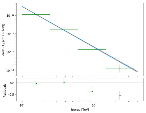
Finally, let’s compute spectral points. The method used is to first choose an energy binning, and then to do a 1-dim likelihood fit / profile to compute the flux and flux error.
In [27]:
# Flux points are computed on stacked observation
stacked_obs = extract.observations.stack()
print(stacked_obs)

ebounds = EnergyBounds.equal_log_spacing(1, 40, 4, unit = u.TeV)

seg = SpectrumEnergyGroupMaker(obs=stacked_obs)
seg.compute_range_safe()
seg.compute_groups_fixed(ebounds=ebounds)

fpe = FluxPointEstimator(
    obs=stacked_obs,
    groups=seg.groups,
    model=fit.result[0].model,
)
fpe.compute_points()
fpe.flux_points.table
WARNING: AstropyDeprecationWarning: The truth value of a Quantity is ambiguous. In the future this will raise a ValueError. [astropy.units.quantity]
WARNING:astropy:AstropyDeprecationWarning: The truth value of a Quantity is ambiguous. In the future this will raise a ValueError.
*** Observation summary report ***
Observation Id: [110380-111159]
Livetime: 1.470 h
On events: 2377
Off events: 34781
Alpha: 0.041
Bkg events in On region: 1432.16
Excess: 944.84
Excess / Background: 0.66
Gamma rate: 0.15 1 / min
Bkg rate: 0.23 1 / min
Sigma: 22.24
energy range: 0.01 TeV - 100.00 TeV
/Users/deil/code/gammapy/gammapy/stats/poisson.py:383: RuntimeWarning: divide by zero encountered in double_scalars
  temp = (alpha + 1) / (n_on + n_off)
/Users/deil/code/gammapy/gammapy/stats/poisson.py:384: RuntimeWarning: divide by zero encountered in log
  l = n_on * log(n_on * temp / alpha)
/Users/deil/code/gammapy/gammapy/stats/fit_statistics.py:161: RuntimeWarning: divide by zero encountered in log
  term2_ = - n_on * np.log(mu_sig + alpha * mu_bkg)
/Users/deil/code/gammapy/gammapy/stats/fit_statistics.py:166: RuntimeWarning: divide by zero encountered in log
  term3_ = - n_off * np.log(mu_bkg)
/Users/deil/code/gammapy/gammapy/stats/fit_statistics.py:203: RuntimeWarning: divide by zero encountered in log
  term1 = - n_on * (1 - np.log(n_on))
/Users/deil/code/gammapy/gammapy/stats/fit_statistics.py:204: RuntimeWarning: divide by zero encountered in log
  term2 = - n_off * (1 - np.log(n_off))
Out[27]:
| e_ref | e_min | e_max | dnde | dnde_err | dnde_ul | is_ul | sqrt_ts | dnde_errp | dnde_errn |
|---|---|---|---|---|---|---|---|---|---|
| TeV | TeV | TeV | 1 / (cm2 s TeV) | 1 / (cm2 s TeV) | 1 / (cm2 s TeV) | 1 / (cm2 s TeV) | 1 / (cm2 s TeV) | ||
| float64 | float64 | float64 | float64 | float64 | float64 | bool | float64 | float64 | float64 |
| 1.56474814166 | 1.0 | 2.44843674682 | 1.09929677082e-12 | 1.23399567803e-13 | 1.36112562438e-12 | False | 13.9252559708 | 1.26220310761e-13 | 1.21722152847e-13 |
| 3.83118684956 | 2.44843674682 | 5.99484250319 | 1.57115663963e-13 | 1.94350698019e-14 | 1.9835646019e-13 | False | 13.6831790276 | 1.98236158774e-14 | 1.86031714233e-14 |
| 9.3804186664 | 5.99484250319 | 14.6779926762 | 1.30447549626e-14 | 3.09086142947e-15 | 2.00964479695e-14 | False | 6.83528872 | 3.32268015634e-15 | 2.88496727552e-15 |
| 22.9673617634 | 14.6779926762 | 35.938136638 | 1.27557550214e-15 | 5.70818610801e-16 | 2.7176911792e-15 | False | 3.55481035321 | 6.49472424329e-16 | 5.04683615003e-16 |
Plot
Let’s plot the spectral model and points. You could do it directly, but there is a helper class. Note that a spectral uncertainty band, a “butterfly” is drawn, but it is very thin, i.e. barely visible.
In [28]:
total_result = SpectrumResult(
    model=fit.result[0].model,
    points=fpe.flux_points,
)

total_result.plot(
    energy_range = [1, 40] * u.TeV,
    fig_kwargs=dict(figsize=(8,8)),
    point_kwargs=dict(color='green'),
)
Out[28]:
(<matplotlib.axes._subplots.AxesSubplot at 0x10b8bebe0>,
 <matplotlib.axes._subplots.AxesSubplot at 0x10b2c67f0>)
Exercises
- Re-run the analysis above, varying some analysis parameters, e.g.
- Select a few other observations
- Change the energy band for the map
- Change the spectral model for the fit
- Change the energy binning for the spectral points
- Change the target. Make a sky image and spectrum for your favourite
source.
- If you don’t know any, the Crab nebula is the “hello world!” analysis of gamma-ray astronomy.
In [29]:
# print('hello world')
# SkyCoord.from_name('crab')
What next?
- This notebook showed an example of a first CTA analysis with Gammapy, using simulated 1DC data.
- This was part 2 for CTA 1DC turorial, the first part was here: cta_1dc_introduction.ipynb
- More tutorials (not 1DC or CTA specific) with Gammapy are here
- Let us know if you have any question or issues!