This is a fixed-text formatted version of a Jupyter notebook.
You can contribute with your own notebooks in this GitHub repository.
Source files: cube_analysis_part1.ipynb | cube_analysis_part1.py
Cube analysis with Gammapy (part 1)
Introduction
In order to run a cube likelihood analysis (combined spectrum and morphology fitting), we first have to prepare the dataset and compute the following inputs by stacking data from observation runs: * counts, background and exposure cube * mean PSF * mean RMF
These are the inputs to the likelihood fitting step, where you assume a parameterised gamma-ray emission model and fit it to the stacked data.
This notebook is part 1 of 2 of a tutorial how to use gammapy.cube to do cube analysis of IACT data. Part 1 is about these pre-computations, part 2 will be about the likelihood fitting.
We will be using the following classes: * gammapy.data.DataStore to load the data to stack in the cube * gammapy.image.SkyImage to work with sky images * gammapy.cube.SkyCube and gammapy.cube.StackedObsCubeMaker to stack the data in the Cube * gammapy.data.ObservationList to make the computation of the mean PSF and mean RMF from a set of runs.
The data used in this tutorial is 4 Crab runs from H.E.S.S..
Setup
As always, we start with some setup for the notebook, and with imports.
In [1]:
%matplotlib inline
import matplotlib.pyplot as plt
In [2]:
import logging
logging.getLogger().setLevel(logging.ERROR)
In [3]:
import numpy as np
import astropy.units as u
from astropy.coordinates import SkyCoord, Angle
from astropy.visualization import simple_norm

from gammapy.data import DataStore
from gammapy.image import SkyImage
from gammapy.cube import SkyCube, StackedObsCubeMaker
Data preparation
Gammapy only supports binned likelihood fits, so we start by defining the spatial and energy grid of the data:
In [4]:
# define WCS specification
WCS_SPEC = {'nxpix': 50,
            'nypix': 50,
            'binsz': 0.05,
            'xref': 83.63,
            'yref': 22.01,
            'proj': 'TAN',
            'coordsys': 'CEL'}

# define reconstructed energy binning
ENERGY_SPEC = {'mode': 'edges',
               'enumbins': 5,
               'emin': 0.5,
               'emax': 40,
               'eunit': 'TeV'}
From this we create an empty SkyCube object, that we will use as
reference for all other sky cube data:
In [5]:
# instanciate reference cube
REF_CUBE = SkyCube.empty(**WCS_SPEC, **ENERGY_SPEC)
Next we create a DataStore object, which allows us to access and
load DL3 level data. In this case we will use four Crab runs of
simulated HESS data, which is bundled in gammapy-extra:
In [6]:
# setting up the data store
data_store = DataStore.from_dir("$GAMMAPY_EXTRA/test_datasets/cube/data")

# temporary fix for load psftable for one of the run that is not implemented yet...
data_store.hdu_table.remove_row(14)
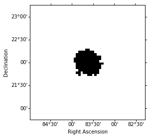
For the later background estimation we define an exclusion mask. The background image will normalized on the counts map outside the exclusion region (the so called FOV background method). For convenience we use and all-sky exclusin mask, which was created from the TeVCat catalog and reproject it to our analysis region:
In [7]:
# read in TeVCat exclusion mask
exclusion_mask = SkyImage.read('$GAMMAPY_EXTRA/datasets/exclusion_masks/tevcat_exclusion.fits')

# reproject exclusion mask to reference cube
exclusion_mask = exclusion_mask.reproject(reference=REF_CUBE.sky_image_ref, order='nearest-neighbor')
That’s what the exclusion mask looks like:
In [8]:
exclusion_mask.show()
Now we can feed all the input to the StackedObsCubeMaker class. In
addition we have to select a offset cut:
In [9]:
#Select the offset band on which you want to select the events in the FOV of each observation
offset_band = Angle([0, 2.49], 'deg')

# instanciate StackedObsCubeMaker
cube_maker = StackedObsCubeMaker(
    empty_cube_images=REF_CUBE,
    empty_exposure_cube=REF_CUBE,
    offset_band=offset_band,
    data_store=data_store,
    obs_table=data_store.obs_table,
    exclusion_mask=exclusion_mask,
    save_bkg_scale=True,
)
We run the cube maker by calling .make_cubes. We pass an correlation
radius of 4 pixels to compute the Li&Ma significance image:
In [10]:
# run cube maker
cube_maker.make_cubes(make_background_image=True, radius=4.)
Let’s take a look at the computed result cubes:
In [11]:
# get counts cube
counts = cube_maker.counts_cube

energies = counts.energies(mode="edges")
print("Bin edges of the count cubes: \n{0}".format(energies))
Bin edges of the count cubes:
[  0.5          1.20112443   2.88539981   6.93144843  16.65106415  40.        ] TeV
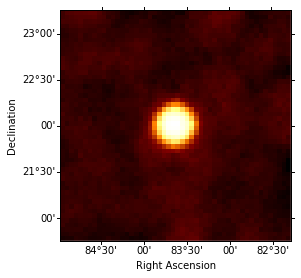
In [12]:
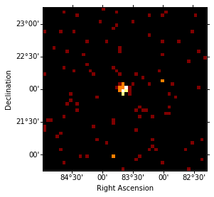
# show counts image with idx = 0
idx = 0
counts.sky_image_idx(idx=idx).show()
print('Energy range: {emin:.2f} to {emax:.2f}'.format(emin=energies[idx], emax=energies[idx + 1]))

Energy range: 0.50 TeV to 1.20 TeV
In [13]:
idx = 3
counts.sky_image_idx(idx=idx).show()
print('Energy range: {emin:.2f} to {emax:.2f}'.format(emin=energies[idx], emax=energies[idx + 1]))
Energy range: 6.93 TeV to 16.65 TeV
In [14]:
background = cube_maker.bkg_cube

idx = 0
background.sky_image_idx(idx=idx).show()
print('Energy range: {emin:.2f} to {emax:.2f}'.format(emin=energies[idx], emax=energies[idx + 1]))
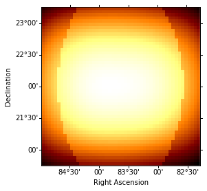
Energy range: 0.50 TeV to 1.20 TeV
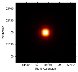
In [15]:
excess = cube_maker.excess_cube

idx = 0
excess.sky_image_idx(idx=idx).show()
print('Energy range: {emin:.2f} to {emax:.2f}'.format(emin=energies[idx], emax=energies[idx + 1]))
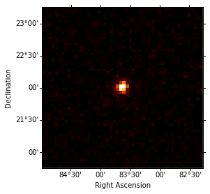
Energy range: 0.50 TeV to 1.20 TeV
In [16]:
significance = cube_maker.significance_cube

idx = 0
significance.sky_image_idx(idx=idx).show()
print('Energy range: {emin:.2f} to {emax:.2f}'.format(emin=energies[idx], emax=energies[idx + 1]))
Energy range: 0.50 TeV to 1.20 TeV
In [17]:
exposure = cube_maker.exposure_cube

idx = 0
exposure.sky_image_idx(idx=idx).show()
print('Energy range: {emin:.2f} to {emax:.2f}'.format(emin=energies[idx], emax=energies[idx + 1]))
Energy range: 0.50 TeV to 1.20 TeV
As a last step we’de like to compute a mean PSF across all observations
in the list. For this purpose we use the .make_mean_psf_cube()
method on the StackedObsCubeMaker object. We only have to specify a
reference cube, which is used to evaluate the PSF model:
In [18]:
with np.errstate(divide='ignore', invalid='ignore'):
    mean_psf_cube = cube_maker.make_mean_psf_cube(REF_CUBE)
Let’s take a quick look a the resulting PSF:
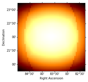
In [19]:
idx = 3
psf_image = mean_psf_cube.sky_image_idx(idx=idx)
norm = simple_norm(psf_image.data, stretch='log')
psf_image.show(norm=norm)
print('Energy range: {emin:.2f} to {emax:.2f}'.format(emin=energies[idx], emax=energies[idx + 1]))
Energy range: 6.93 TeV to 16.65 TeV
Now we repeat the computation but assume a different energy binning for the “true” energy:
In [20]:
# define true energy binning
ENERGY_TRUE_SPEC = {'mode': 'edges',
                    'enumbins': 20,
                    'emin': 0.1,
                    'emax': 100,
                    'eunit': 'TeV'}

# init refereence cube
REF_CUBE_TRUE = SkyCube.empty(**WCS_SPEC, **ENERGY_TRUE_SPEC)
The reference cube is now passed to the empty_exposure_cube
argument:
In [21]:
cube_maker = StackedObsCubeMaker(
    empty_cube_images=REF_CUBE,
    empty_exposure_cube=REF_CUBE_TRUE,
    offset_band=offset_band,
    data_store=data_store,
    obs_table=data_store.obs_table,
    exclusion_mask=exclusion_mask,
    save_bkg_scale=True,
)
cube_maker.make_cubes(make_background_image=True, radius=10.)
The PSF can computed using the “true” energy reference cube as well:
In [22]:
with np.errstate(divide='ignore', invalid='ignore'):
    mean_psf_cube = cube_maker.make_mean_psf_cube(REF_CUBE_TRUE)
In [23]:
e_reco = cube_maker.counts_cube.energies(mode="edges")
print("Energy bin edges of the count cube: \n{}\n".format(e_reco))

e_true = cube_maker.exposure_cube.energies(mode="edges")
print("Energy bin edges of the exposure cube: \n{}".format(e_true))
Energy bin edges of the count cube:
[  0.5          1.20112443   2.88539981   6.93144843  16.65106415  40.        ] TeV

Energy bin edges of the exposure cube:
[  1.00000000e-01   1.41253754e-01   1.99526231e-01   2.81838293e-01
   3.98107171e-01   5.62341325e-01   7.94328235e-01   1.12201845e+00
   1.58489319e+00   2.23872114e+00   3.16227766e+00   4.46683592e+00
   6.30957344e+00   8.91250938e+00   1.25892541e+01   1.77827941e+01
   2.51188643e+01   3.54813389e+01   5.01187234e+01   7.07945784e+01
   1.00000000e+02] TeV
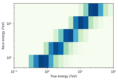
Finally we compute the mean RMF (energy dispersion matrix) across multiple observations:
In [24]:
# get reference energies
obs_list = data_store.obs_list(data_store.obs_table['OBS_ID'])
position = REF_CUBE.sky_image_ref.center
e_true = REF_CUBE_TRUE.energies('edges')
e_reco = REF_CUBE.energies('edges')

with np.errstate(divide='ignore', invalid='ignore'):
    mean_rmf = obs_list.make_mean_edisp(position=position, e_true=e_true, e_reco=e_reco)
In [25]:
mean_rmf.plot_matrix()
/opt/local/Library/Frameworks/Python.framework/Versions/3.5/lib/python3.5/site-packages/matplotlib/colors.py:1152: UserWarning: Power-law scaling on negative values is ill-defined, clamping to 0.
  warnings.warn("Power-law scaling on negative values is "
Out[25]:
<matplotlib.axes._subplots.AxesSubplot at 0x10e0ecef0>
/opt/local/Library/Frameworks/Python.framework/Versions/3.5/lib/python3.5/site-packages/matplotlib/colors.py:1113: RuntimeWarning: invalid value encountered in power
  np.power(resdat, gamma, resdat)
Exercises
- Take another dataset
- Change the Cube binning
Now that we created some cubes for counts, background, exposure, psf from a set of runs we will learn in the future tutorials how to use it for a 3D analysis (morphological and spectral)