This is a fixed-text formatted version of a Jupyter notebook.

You can contribute with your own notebooks in this GitHub repository.

Source files: image_pipe.ipynb | image_pipe.py

Image analysis with Gammapy (run pipeline)¶

In this tutorial we’ll learn how to make 2-dimensional images with Gammapy: counts, background, excess, significance, exposure and flux.

We will use a “pipeline” or “workflow” class, the StackedObsImageMaker, that takes the inputs and some parameters as input, and then computes all images when we call the make_images method, i.e. without us having to write a lot code or know how it’s implemented.

There’s another tutorial (image_analysis.ipynb) that executes the analysis using lower-level classes and methods in Gammapy. That other notebook would be useful to you if you’d like to understand what method is executed, or if you’d like to tweak it for your use case.

In this tutorial we will use the folling Gammapy classes:

gammapy.data.DataStore to load the data to stack in the images
gammapy.image.SkyImage for the sky images (counts, background, exclusion, …)
gammapy.scripts.StackedObsImageMaker to create the images

We use 4 Crab observations from H.E.S.S. for testing.

Setup¶

As usual, we’ll start with some setup for the notebook, and import the functionality we need.

In [1]:

%matplotlib inline
import numpy as np
import matplotlib.pyplot as plt

In [2]:

import astropy.units as u
from astropy.coordinates import SkyCoord, Angle
from astropy.table import Table
from astropy.visualization import simple_norm

from gammapy.data import DataStore
from gammapy.image import SkyImage
from gammapy.scripts import StackedObsImageMaker
from gammapy.utils.energy import Energy

Define inputs¶

We start by defining the inputs to use for the analysis:

which data and instrument response functions to use
sky image geometry
energy band
maximum field of view offset cut

The data (events, background models, effective area for exposure computation) consist of a few H.E.S.S. Crab observation runs as example. The background models there were produced as explained in the background_model.ipynb tutorial.

In [3]:

# What data to analyse
data_store = DataStore.from_dir('$GAMMAPY_EXTRA/test_datasets/cube/data')
# Define runlist
obs_table = Table()
obs_table['OBS_ID'] = [23523, 23526, 23592]
# There's a problem with the PSF for run 23559, so we don't use that run for now.

In [4]:

# Define sky image
ref_image = SkyImage.empty(
    nxpix=300, nypix=300, binsz=0.02,
    xref=83.63, yref=22.01,
    proj='TAN', coordsys='CEL',
)

In [5]:

# Define energy band
energy_band = Energy([1, 10], 'TeV')

In [6]:

# Define maximum field of view offset cut
offset_band = Angle([0, 2.49], 'deg')

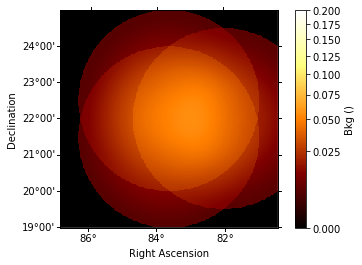
You define an exclusion mask that will be use to create the backgroud 2D map. The background map are normalized on the counts map outside the exclusion region

In [7]:

# Define exclusion mask (known gamma-ray sources)
# This is used in the background model image estimation
exclusion_mask = SkyImage.read('$GAMMAPY_EXTRA/datasets/exclusion_masks/tevcat_exclusion.fits')
exclusion_mask = exclusion_mask.reproject(reference=ref_image)

# If you don't have an exclusion mask,
# you could also start with an empty one
# exclusion_mask = SkyImage.empty_like(ref_image)

Make the images¶

To make the images, we just pass the inputs to StackedObsImageMaker and then call the make_images method. Creating the StackedObsImageMaker doesn’t do any computations, it just stores the parts as data members, all the computation happens in the make_images method.

In [8]:

image_maker = StackedObsImageMaker(
    empty_image=ref_image,
    energy_band=energy_band,
    offset_band=offset_band,
    data_store=data_store,
    obs_table=obs_table,
    exclusion_mask=exclusion_mask,
)

In [9]:

image_maker.make_images(
    make_background_image=True,
    for_integral_flux=True,
    radius=4,
)

WARNING:gammapy.irf.psf_analytical:No safe energy thresholds found. Setting to default
WARNING:gammapy.irf.psf_king:No safe energy thresholds found. Setting to default
WARNING:gammapy.irf.psf_king:No safe energy thresholds found. Setting to default
/Users/deil/Library/Python/3.5/lib/python/site-packages/gammapy-0.6.dev4380-py3.5-macosx-10.12-x86_64.egg/gammapy/stats/poisson.py:254: RuntimeWarning: divide by zero encountered in true_divide
  term_b = sqrt(n_on * log(n_on / mu_bkg) - n_on + mu_bkg)

Check the results¶

The resulting sky images are stored in the image_maker.images property.

Let’s have a look …

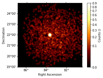
Counts image¶

In [10]:

counts_image = image_maker.images['counts']
norm = simple_norm(counts_image.data, stretch='sqrt', min_cut=0, max_cut=0.9)
counts_image.smooth(radius=0.08 * u.deg).plot(norm=norm, add_cbar=True)

Out[10]:

(<matplotlib.figure.Figure at 0x10f1d2358>,
 <matplotlib.axes._subplots.WCSAxesSubplot at 0x1153032e8>,
 <matplotlib.colorbar.Colorbar at 0x1155a1940>)

../_images/notebooks_image_pipe_17_1.png

Background Image¶

In [11]:

background_image = image_maker.images['bkg']
norm = simple_norm(background_image.data, stretch='sqrt', min_cut=0, max_cut=0.2)
background_image.plot(norm=norm, add_cbar=True)

Out[11]:

(<matplotlib.figure.Figure at 0x1155bcf60>,
 <matplotlib.axes._subplots.WCSAxesSubplot at 0x10f1d2128>,
 <matplotlib.colorbar.Colorbar at 0x10f19fcf8>)

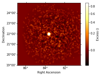
../_images/notebooks_image_pipe_19_1.png

Excess Image¶

In [12]:

excess_image = image_maker.images['excess']
norm = simple_norm(excess_image.data, stretch='sqrt', min_cut=0, max_cut=0.9)
excess_image.smooth(radius=0.08 * u.deg).plot(norm=norm,add_cbar=True)

Out[12]:

(<matplotlib.figure.Figure at 0x111cd1898>,
 <matplotlib.axes._subplots.WCSAxesSubplot at 0x1155c82e8>,
 <matplotlib.colorbar.Colorbar at 0x1150c4f98>)

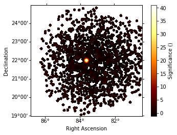
../_images/notebooks_image_pipe_21_1.png

Significance Image¶

In [13]:

# Looks like a leopard, because pixels with `NaN`
# values are shown in white,
image_maker.images["significance"].plot(add_cbar=True)

Out[13]:

(<matplotlib.figure.Figure at 0x11228f940>,
 <matplotlib.axes._subplots.WCSAxesSubplot at 0x1151ccfd0>,
 <matplotlib.colorbar.Colorbar at 0x115c3d0f0>)

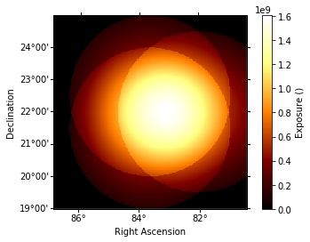
../_images/notebooks_image_pipe_23_1.png

Exposure Image¶

In [14]:

image_maker.images["exposure"].plot(add_cbar=True)

Out[14]:

(<matplotlib.figure.Figure at 0x115c4e0f0>,
 <matplotlib.axes._subplots.WCSAxesSubplot at 0x115c4b358>,
 <matplotlib.colorbar.Colorbar at 0x1161b66a0>)

../_images/notebooks_image_pipe_25_1.png

Exercises¶

For the output image, create a cutout zooming in on the Crab nebula, and add a marker at the Crab pulsar position
Change the energy band to something else you like and re-run the whole analysis
Change the sky image to Galactic coordinates and re-run the analysis
Change the maximum FOV offset cut to something smaller (e.g. 1.5 deg) and re-run the analysis

Navigation