This is a fixed-text formatted version of a Jupyter notebook.

You can contribute with your own notebooks in this GitHub repository.

Source files: spectrum_simulation_cta.ipynb | spectrum_simulation_cta.py

Spectrum simulation for CTA¶

A quick example how to simulate and fit a spectrum for the Cherenkov Telescope Array (CTA)

We will use the following classes:

Setup¶

In [1]:

%matplotlib inline
import matplotlib.pyplot as plt

In [2]:

import numpy as np
import astropy.units as u
from gammapy.irf import EnergyDispersion, EffectiveAreaTable
from gammapy.spectrum import SpectrumSimulation, SpectrumFit
from gammapy.spectrum.models import PowerLaw
from gammapy.scripts import CTAIrf

Simulation¶

In [3]:

# Define obs parameters
livetime = 10 * u.min
offset = 0.3 * u.deg
lo_threshold = 0.1 * u.TeV
hi_threshold = 60 * u.TeV

In [4]:

# Define spectral model
index = 2.3 * u.Unit('')
amplitude = 2.5 * 1e-12 * u.Unit('cm-2 s-1 TeV-1')
reference = 1 * u.TeV
model = PowerLaw(index=index, amplitude=amplitude, reference=reference)

In [5]:

# Load IRFs
filename = '$GAMMAPY_EXTRA/datasets/cta/perf_prod2/South_5h/irf_file.fits.gz'
cta_irf = CTAIrf.read(filename)

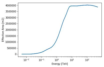
In [6]:

aeff = cta_irf.aeff.to_effective_area_table(offset=offset)
aeff.plot()
print(cta_irf.aeff.data)

NDDataArray summary info
energy         : size =   500, min =  0.005 TeV, max = 495.450 TeV
offset         : size =    45, min =  0.050 deg, max =  4.450 deg
Data           : size = 22500, min =  0.000 m2, max = 4033200.000 m2

../_images/notebooks_spectrum_simulation_cta_9_1.png

In [7]:

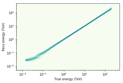
edisp = cta_irf.edisp.to_energy_dispersion(offset=offset)
edisp.plot_matrix()
print(edisp.data)

/Users/deil/Library/Python/3.6/lib/python/site-packages/astropy-2.0.dev18336-py3.6-macosx-10.12-x86_64.egg/astropy/units/quantity.py:1005: RuntimeWarning: invalid value encountered in true_divide
  return super(Quantity, self).__truediv__(other)

NDDataArray summary info
e_true         : size =   500, min =  0.005 TeV, max = 495.450 TeV
e_reco         : size =   500, min =  0.005 TeV, max = 495.450 TeV
Data           : size = 250000, min =  0.000, max =  0.165

../_images/notebooks_spectrum_simulation_cta_10_2.png

In [8]:

# Simulate data
aeff.lo_threshold = lo_threshold
aeff.hi_threshold = hi_threshold
sim = SpectrumSimulation(aeff=aeff, edisp=edisp, source_model=model, livetime=livetime)
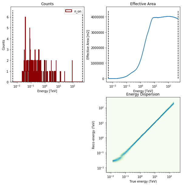
sim.simulate_obs(seed=42, obs_id=0)

In [9]:

sim.obs.peek()
print(sim.obs)

/Users/deil/Library/Python/3.6/lib/python/site-packages/gammapy-0.7.dev4616-py3.6-macosx-10.12-x86_64.egg/gammapy/data/obs_stats.py:209: RuntimeWarning: divide by zero encountered in true_divide
  self.background))
/Users/deil/Library/Python/3.6/lib/python/site-packages/gammapy-0.7.dev4616-py3.6-macosx-10.12-x86_64.egg/gammapy/stats/poisson.py:385: RuntimeWarning: divide by zero encountered in log
  m = n_off * log(n_off * temp)
/Users/deil/Library/Python/3.6/lib/python/site-packages/gammapy-0.7.dev4616-py3.6-macosx-10.12-x86_64.egg/gammapy/stats/poisson.py:385: RuntimeWarning: invalid value encountered in multiply
  m = n_off * log(n_off * temp)

*** Observation summary report ***
Observation Id: 0
Livetime: 0.167 h
On events: 165
Off events: 0
Alpha: 1.000
Bkg events in On region: 0.00
Excess: 165.00
Excess / Background: inf
Gamma rate: 0.03 1 / min
Bkg rate: 0.00 1 / min
Sigma: nan
energy range: 0.01 TeV - 501.19 TeV

../_images/notebooks_spectrum_simulation_cta_12_2.png

Spectral analysis¶

Now that we have some simulated CTA counts spectrum, let’s analyse it.

In [10]:

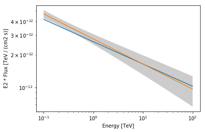
# Fit data
fit = SpectrumFit(obs_list=sim.obs, model=model, stat='cash')
fit.run()
result = fit.result[0]

INFO:gammapy.spectrum.fit:Running SpectrumFit
Source model PowerLaw

Parameters:

           name     value   error       unit      min  max  frozen
        --------- --------- ----- --------------- ---- ---- ------
            index 2.300e+00   nan                    0 None  False
        amplitude 2.500e-12   nan 1 / (cm2 s TeV)    0 None  False
        reference 1.000e+00   nan             TeV None None   True
Stat cash
Forward Folded True
Fit range None
Backend sherpa
Error Backend sherpa
/Users/deil/Library/Python/3.6/lib/python/site-packages/gammapy-0.7.dev4616-py3.6-macosx-10.12-x86_64.egg/gammapy/stats/fit_statistics.py:55: RuntimeWarning: divide by zero encountered in log
  stat = 2 * (mu_on - n_on * np.log(mu_on))

In [11]:

print(result)


Fit result info
---------------
Model: PowerLaw

Parameters:

           name     value     error         unit      min  max  frozen
        --------- --------- --------- --------------- ---- ---- ------
            index 2.229e+00 4.879e-02                    0 None  False
        amplitude 2.774e-12 2.984e-13 1 / (cm2 s TeV)    0 None  False
        reference 1.000e+00 0.000e+00             TeV None None   True

Covariance:

        name/name  index  amplitude
        --------- ------- ---------
            index 0.00238    -1e-14
        amplitude  -1e-14   8.9e-26

Statistic: 460.387 (cash)
Fit Range: [  5.01187239e-03   5.01187225e+02] TeV

In [12]:

energy_range = [0.1, 100] * u.TeV
model.plot(energy_range=energy_range, energy_power=2)
result.model.plot(energy_range=energy_range, energy_power=2)
result.model.plot_error(energy_range=energy_range, energy_power=2)

Out[12]:

<matplotlib.axes._subplots.AxesSubplot at 0x10d933710>

../_images/notebooks_spectrum_simulation_cta_16_1.png

Exercises¶

Change the observation time to something longer or shorter. Does the observation and spectrum results change as you expected?
Change the spectral model, e.g. add a cutoff at 5 TeV, or put a steep-spectrum source with spectral index of 4.0

In [13]:

# Start the exercises here!

What next?¶

In this tutorial we simulated and analysed the spectrum of source using CTA prod 2 IRFs.

If you’d like to go further, please see the other tutorial notebooks.