This is a fixed-text formatted version of a Jupyter notebook.
You can contribute with your own notebooks in this GitHub repository.
Source files: astropy_introduction.ipynb | astropy_introduction.py
Astropy introduction for Gammapy users
Introduction
To become efficient at using Gammapy, you have to learn to use some parts of Astropy, especially FITS I/O and how to work with Table, Quantity, SkyCoord, Angle and Time objects.
Gammapy is built on Astropy, meaning that data in Gammapy is often stored in Astropy objects, and the methods on those objects are part of the public Gammapy API.
This tutorial is a quick introduction to the parts of Astropy you should know become familiar with to use Gammapy (or also when not using Gammapy, just doing astronomy from Python scripts). The largest part is devoted to tables, which are a the most important building block for Gammapy (event lists, flux points, light curves, … many other thing are store in Table objects).
We will:
- open and write fits files with io.fits
- manipulate coordinates: SkyCoord and Angle classes
- use units and Quantities. See also this tutorial
- manipulate Times and Dates
- use tables with the Table class with the Fermi catalog
- define regions in the sky with the region package
Setup
In [1]:
# to make plots appear in the notebook
%matplotlib inline
import matplotlib.pyplot as plt
In [2]:
# If something below doesn't work, here's how you
# can check what version of Numpy and Astropy you have
# All examples should work with Astropy 1.3,
# most even with Astropy 1.0
import numpy as np
import astropy
print('numpy:', np.__version__)
print('astropy:', astropy.__version__)
numpy: 1.12.1
astropy: 2.0.dev17848
In [3]:
# Units, Quantities and constants
import astropy.units as u
from astropy.units import Quantity
import astropy.constants as cst

from astropy.io import fits
from astropy.table import Table
from astropy.coordinates import SkyCoord, Angle
from astropy.time import Time
Units and constants
Basic usage
In [4]:
# One can create a Quantity like this
L = Quantity(1e35, unit='erg/s')
# or like this
d = 8 * u.kpc

# then one can produce new Quantities
flux = L / (4 * np.pi * d ** 2)

# And convert its value to any (homogeneous) unit
print(flux.to('erg cm-2 s-1'))
print(flux.to('W/m2'))
# print(flux.to('Ci')) would raise a UnitConversionError
1.3058974431347377e-11 erg / (cm2 s)
1.3058974431347378e-14 W / m2
More generally a Quantity is a numpy array with a unit.
In [5]:
E = np.logspace(1, 4, 10) * u.GeV
print(E.to('TeV'))
[  0.01         0.02154435   0.04641589   0.1          0.21544347
   0.46415888   1.           2.15443469   4.64158883  10.        ] TeV
Here we compute the interaction time of protons.
In [6]:
x_eff = 30 * u.mbarn
density = 1 * u.cm ** -3

interaction_time = (density * x_eff * cst.c) ** -1

interaction_time.to('Myr')
Out[6]:
Use Quantities in functions
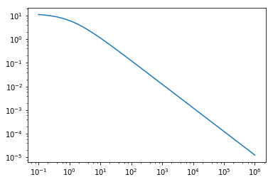
We compute here the energy loss rate of an electron of kinetic energy E in magnetic field B. See formula (5B10) in this lecture
In [7]:
def electron_energy_loss_rate(B, E):
    """ energy loss rate of an electron of kinetic energy E in magnetic field B
    """
    U_B = B ** 2 / (2 * cst.mu0)
    gamma = E / (cst.m_e * cst.c ** 2) + 1   # note that this works only because E/(cst.m_e*cst.c**2) is dimensionless
    beta = np.sqrt(1 - 1 / gamma ** 2)
    return 4. / 3. * cst.sigma_T * cst.c * gamma ** 2 * beta ** 2 * U_B

print(electron_energy_loss_rate(1e-5 * u.G, 1 * u.TeV).to('erg/s'))

# Now plot it
E_elec = np.logspace(-1., 6, 100) * u.MeV
B = 1 * u.G
plt.loglog(E_elec,(E_elec / electron_energy_loss_rate(B, E_elec)).to('yr'))
4.0519328131469305e-13 erg / s
Out[7]:
[<matplotlib.lines.Line2D at 0x10b2ee048>]
A frequent issue is homogeneity. One can use decorators to ensure it.
In [8]:
# This ensures that B and E are homogeneous to magnetic field strength and energy
# If not will raise a UnitError exception
@u.quantity_input(B=u.T,E=u.J)
def electron_energy_loss_rate(B, E):
    """ energy loss rate of an electron of kinetic energy E in magnetic field B
    """
    U_B = B ** 2 / (2 * cst.mu0)
    gamma = E / (cst.m_e * cst.c ** 2) + 1   # note that this works only because E/(cst.m_e*cst.c**2) is dimensionless
    beta = np.sqrt(1 - 1 / gamma ** 2)
    return 4. / 3. * cst.sigma_T * cst.c * gamma ** 2 * beta ** 2 * U_B

# Now try it
try:
    print(electron_energy_loss_rate(1e-5 * u.G, 1 * u.Hz).to('erg/s'))
except u.UnitsError as message:
    print('Incorrect unit: '+ str(message))
Incorrect unit: Argument 'E' to function 'electron_energy_loss_rate' must be in units convertible to 'J'.
Coordinates
Note that SkyCoord are arrays of coordinates. We will see that in more detail in the next section.
In [9]:
# Different ways to create a SkyCoord
c1 = SkyCoord(10.625, 41.2, frame='icrs', unit='deg')
c1 = SkyCoord('00h42m30s', '+41d12m00s', frame='icrs')

c2 = SkyCoord(83.633083, 22.0145, unit='deg')
# If you have internet access, you could also use this to define the `source_pos`:
# c2 = SkyCoord.from_name("Crab")     # Get the name from CDS

print(c1.ra,c2.dec)

print('Distance to Crab: ', c1.separation(c2))    # separation returns an Angle object
print('Distance to Crab: ', c1.separation(c2).degree)
10d37m30s 22d00m52.2s
Distance to Crab:  63d12m28.2297s
Distance to Crab:  63.2078415848386
Coordinate transformations
How to change between coordinate frames. The Crab in Galactic coordinates.
In [10]:
c2b = c2.galactic
print(c2b)
print(c2b.l, c2b.b)
<SkyCoord (Galactic): (l, b) in deg
    ( 184.55745771, -5.78435696)>
184d33m26.8478s -5d47m03.6851s
Time
Is the Crab visible now?
In [11]:
now = Time.now()
print(now)
print(now.mjd)
2017-04-11 06:58:46.032083
57854.290810556515
In [12]:
# define the location for the AltAz system
from astropy.coordinates import EarthLocation, AltAz
paris = EarthLocation(lat=48.8567 * u.deg, lon=2.3508 * u.deg )

# calculate the horizontal coordinates
crab_altaz = c2.transform_to(AltAz(obstime=now, location=paris))

print(crab_altaz)
<SkyCoord (AltAz: obstime=2017-04-11 06:58:46.032083, location=(4200910.643257838, 172456.78503911156, 4780088.658775934) m, pressure=0.0 hPa, temperature=0.0 deg_C, relative_humidity=0, obswl=1.0 micron): (az, alt) in deg
    ( 39.72687934, -9.48762642)>
Table: Manipulating the 3FGL catalog
Here we are going to do some selections with the 3FGL catalog. To do so we use the Table class from astropy.
Accessing the table
First, we need to open the catalog in a Table.
In [13]:
# Open Fermi 3FGL from the repo
table = Table.read("../datasets/catalogs/fermi/gll_psc_v16.fit.gz")
# Alternatively, one can grab it from the server.
#table = Table.read("http://fermi.gsfc.nasa.gov/ssc/data/access/lat/4yr_catalog/gll_psc_v16.fit")
WARNING: hdu= was not specified but multiple tables are present, reading in first available table (hdu=1) [astropy.io.fits.connect]
WARNING: UnitsWarning: 'photon/cm**2/MeV/s' contains multiple slashes, which is discouraged by the FITS standard [astropy.units.format.generic]
WARNING: UnitsWarning: 'photon/cm**2/s' contains multiple slashes, which is discouraged by the FITS standard [astropy.units.format.generic]
WARNING: UnitsWarning: The unit 'erg' has been deprecated in the FITS standard. Suggested: cm2 g s-2. [astropy.units.format.utils]
WARNING: UnitsWarning: 'erg/cm**2/s' contains multiple slashes, which is discouraged by the FITS standard [astropy.units.format.generic]
In [14]:
# Note that a single FITS file might contain different tables in different HDUs
filename = "../datasets/catalogs/fermi/gll_psc_v16.fit.gz"
# You can load a `fits.HDUList` and check the extension names
print([_.name for _ in fits.open(filename)])
# Then you can load by name or integer index via the `hdu` option
extended_source_table = Table.read(filename, hdu='ExtendedSources')
['PRIMARY', 'LAT_Point_Source_Catalog', 'ROIs', 'Hist_Start', 'GTI', 'ExtendedSources']
General informations on the Table
In [15]:
table.info()
<Table length=3034>
        name          dtype   shape        unit       n_bad
-------------------- ------- ------- ---------------- -----
         Source_Name   str18                              0
             RAJ2000 float32                      deg     0
             DEJ2000 float32                      deg     0
                GLON float32                      deg     0
                GLAT float32                      deg     0
   Conf_68_SemiMajor float32                      deg    28
   Conf_68_SemiMinor float32                      deg    28
      Conf_68_PosAng float32                      deg    28
   Conf_95_SemiMajor float32                      deg    28
   Conf_95_SemiMinor float32                      deg    28
      Conf_95_PosAng float32                      deg    28
             ROI_num   int16                              0
          Signif_Avg float32                              5
        Pivot_Energy float32                      MeV     0
        Flux_Density float32         ph / (cm2 MeV s)     0
    Unc_Flux_Density float32         ph / (cm2 MeV s)     5
            Flux1000 float32             ph / (cm2 s)     0
        Unc_Flux1000 float32             ph / (cm2 s)     5
      Energy_Flux100 float32            erg / (cm2 s)     0
  Unc_Energy_Flux100 float32            erg / (cm2 s)     5
        Signif_Curve float32                              0
        SpectrumType   str16                              0
      Spectral_Index float32                              0
  Unc_Spectral_Index float32                              9
                beta float32                           2639
            Unc_beta float32                           2680
              Cutoff float32                      MeV  2918
          Unc_Cutoff float32                      MeV  2918
           Exp_Index float32                           2918
       Unc_Exp_Index float32                           3028
      PowerLaw_Index float32                              0
          Flux30_100 float32             ph / (cm2 s)  3034
      Unc_Flux30_100 float32             ph / (cm2 s)  3034
         nuFnu30_100 float32            erg / (cm2 s)  3034
       Sqrt_TS30_100 float32                           3034
         Flux100_300 float32             ph / (cm2 s)     0
     Unc_Flux100_300 float32    (2,)     ph / (cm2 s)   836
        nuFnu100_300 float32            erg / (cm2 s)     0
      Sqrt_TS100_300 float32                              5
        Flux300_1000 float32             ph / (cm2 s)     0
    Unc_Flux300_1000 float32    (2,)     ph / (cm2 s)   327
       nuFnu300_1000 float32            erg / (cm2 s)     0
     Sqrt_TS300_1000 float32                              5
       Flux1000_3000 float32             ph / (cm2 s)     0
   Unc_Flux1000_3000 float32    (2,)     ph / (cm2 s)   111
      nuFnu1000_3000 float32            erg / (cm2 s)     0
    Sqrt_TS1000_3000 float32                              0
      Flux3000_10000 float32             ph / (cm2 s)     0
  Unc_Flux3000_10000 float32    (2,)     ph / (cm2 s)   137
     nuFnu3000_10000 float32            erg / (cm2 s)     0
   Sqrt_TS3000_10000 float32                              3
    Flux10000_100000 float32             ph / (cm2 s)     0
Unc_Flux10000_100000 float32    (2,)     ph / (cm2 s)   670
   nuFnu10000_100000 float32            erg / (cm2 s)     0
 Sqrt_TS10000_100000 float32                              2
   Variability_Index float32                              0
         Signif_Peak float32                           2387
           Flux_Peak float32             ph / (cm2 s)  2387
       Unc_Flux_Peak float32             ph / (cm2 s)  2387
           Time_Peak float64                        s  2387
       Peak_Interval float32                        s  2387
        Flux_History float32   (48,)     ph / (cm2 s)     0
    Unc_Flux_History float32 (48, 2)     ph / (cm2 s) 64623
Extended_Source_Name   str18                              0
           0FGL_Name   str17                              0
           1FGL_Name   str18                              0
           2FGL_Name   str18                              0
           1FHL_Name   str18                              0
          ASSOC_GAM1   str15                              0
          ASSOC_GAM2   str14                              0
          ASSOC_GAM3   str15                              0
         TEVCAT_FLAG    str1                              0
           ASSOC_TEV   str21                              0
              CLASS1    str5                              0
              ASSOC1   str26                              0
              ASSOC2   str26                              0
               Flags   int16                              0
In [16]:
# Statistics on each column
table.info('stats')
<Table length=3034>
        name              mean          std          min         max     n_bad
-------------------- ------------- ------------- ----------- ----------- -----
         Source_Name            --            --          --          --     0
             RAJ2000       185.638       100.585      0.0377     359.881     0
             DEJ2000      -2.23514       41.5371    -87.6185     88.7739     0
                GLON       186.273       107.572    0.126161     359.969     0
                GLAT       1.22728       36.4998    -87.9516     86.3679     0
   Conf_68_SemiMajor          -inf           nan        -inf    0.658726    28
   Conf_68_SemiMinor          -inf           nan        -inf    0.320945    28
      Conf_68_PosAng     -0.219671       51.9263      -89.94       89.92    28
   Conf_95_SemiMajor          -inf           nan        -inf      1.0681    28
   Conf_95_SemiMinor          -inf           nan        -inf      0.5204    28
      Conf_95_PosAng     -0.219671       51.9263      -89.94       89.92    28
             ROI_num 424.777191826 238.846231996           1         840     0
          Signif_Avg          -inf           nan        -inf     1048.96     5
        Pivot_Energy       2104.46        2578.2     100.798     37202.0     0
        Flux_Density   1.29389e-11   2.17231e-10 4.21515e-16 1.14476e-08     0
    Unc_Flux_Density          -inf           nan        -inf 6.86476e-10     5
            Flux1000    2.7507e-09   2.76475e-08 4.90582e-12 1.29768e-06     0
        Unc_Flux1000          -inf           nan        -inf 2.89396e-09     5
      Energy_Flux100   2.56011e-11   1.88859e-10 1.65227e-12 8.93008e-09     0
  Unc_Energy_Flux100          -inf           nan        -inf 2.52953e-11     5
        Signif_Curve       2.43161       3.87731         0.0      84.973     0
        SpectrumType            --            --          --          --     0
      Spectral_Index       2.21451      0.360539         0.5     5.71589     0
  Unc_Spectral_Index          -inf           nan        -inf     1.06113     9
                beta          -inf           nan        -inf         1.0  2639
            Unc_beta          -inf           nan        -inf    0.337608  2680
              Cutoff          -inf           nan        -inf     13326.4  2918
          Unc_Cutoff          -inf           nan        -inf     3750.56  2918
           Exp_Index          -inf           nan        -inf         1.0  2918
       Unc_Exp_Index          -inf           nan        -inf   0.0442999  3028
      PowerLaw_Index       2.24982      0.306354     1.09753     5.71589     0
          Flux30_100           nan           nan         nan         nan  3034
      Unc_Flux30_100           nan           nan         nan         nan  3034
         nuFnu30_100           nan           nan         nan         nan  3034
       Sqrt_TS30_100           nan           nan         nan         nan  3034
         Flux100_300   2.37795e-08   1.20342e-07 1.00222e-14 5.37625e-06     0
     Unc_Flux100_300          -inf           nan        -inf 9.56701e-08   836
        nuFnu100_300   5.71922e-12   3.02685e-11 2.49123e-18 1.37177e-09     0
      Sqrt_TS100_300       3.81654       8.91583         0.0     215.416     5
        Flux300_1000   8.61936e-09   6.73293e-08 3.97788e-15 3.21672e-06     0
    Unc_Flux300_1000          -inf           nan        -inf 1.89716e-08   327
       nuFnu300_1000   5.90484e-12   4.79845e-11 2.91179e-18 2.29243e-09     0
     Sqrt_TS300_1000        7.4718       19.8981         0.0     568.663     5
       Flux1000_3000   2.19502e-09   2.27795e-08 1.50877e-15 1.07019e-06     0
   Unc_Flux1000_3000          -inf           nan        -inf 6.09948e-09   111
      nuFnu1000_3000   5.14613e-12   5.38784e-11 3.76523e-18 2.52534e-09     0
    Sqrt_TS1000_3000       8.60778       22.2479         0.0     711.632     0
      Flux3000_10000   4.83629e-10   4.64785e-09 9.33897e-16 2.16177e-07     0
  Unc_Flux3000_10000          -inf           nan        -inf 2.98606e-09   137
     nuFnu3000_10000   3.07335e-12   2.83225e-11  5.6769e-18 1.32102e-09     0
   Sqrt_TS3000_10000       6.98671       13.9194         0.0     465.899     3
    Flux10000_100000   7.39921e-11   3.22538e-10 1.03878e-17 1.13815e-08     0
Unc_Flux10000_100000          -inf           nan        -inf 7.88092e-10   670
   nuFnu10000_100000   1.16414e-12   4.63575e-12 9.38528e-20 1.16018e-10     0
 Sqrt_TS10000_100000       4.01938       5.47004         0.0     111.192     2
   Variability_Index       154.126       1230.71         0.0     60733.9     0
         Signif_Peak          -inf           nan        -inf     255.071  2387
           Flux_Peak          -inf           nan        -inf 2.12374e-05  2387
       Unc_Flux_Peak          -inf           nan        -inf 1.47859e-07  2387
           Time_Peak          -inf           nan        -inf 364203776.0  2387
       Peak_Interval          -inf           nan        -inf    2.63e+06  2387
        Flux_History   3.54401e-08   2.26052e-07         0.0 2.12374e-05     0
    Unc_Flux_History          -inf           nan        -inf 2.30386e-07 64623
Extended_Source_Name            --            --          --          --     0
           0FGL_Name            --            --          --          --     0
           1FGL_Name            --            --          --          --     0
           2FGL_Name            --            --          --          --     0
           1FHL_Name            --            --          --          --     0
          ASSOC_GAM1            --            --          --          --     0
          ASSOC_GAM2            --            --          --          --     0
          ASSOC_GAM3            --            --          --          --     0
         TEVCAT_FLAG            --            --          --          --     0
           ASSOC_TEV            --            --          --          --     0
              CLASS1            --            --          --          --     0
              ASSOC1            --            --          --          --     0
              ASSOC2            --            --          --          --     0
               Flags 45.7735662492 265.711605004           0        2565     0
/opt/local/Library/Frameworks/Python.framework/Versions/3.5/lib/python3.5/site-packages/numpy/lib/nanfunctions.py:1304: RuntimeWarning: invalid value encountered in subtract
  np.subtract(arr, avg, out=arr, casting='unsafe')
/opt/local/Library/Frameworks/Python.framework/Versions/3.5/lib/python3.5/site-packages/numpy/lib/nanfunctions.py:1304: RuntimeWarning: invalid value encountered in subtract
  np.subtract(arr, avg, out=arr, casting='unsafe')
/opt/local/Library/Frameworks/Python.framework/Versions/3.5/lib/python3.5/site-packages/numpy/lib/nanfunctions.py:1304: RuntimeWarning: invalid value encountered in subtract
  np.subtract(arr, avg, out=arr, casting='unsafe')
/opt/local/Library/Frameworks/Python.framework/Versions/3.5/lib/python3.5/site-packages/numpy/lib/nanfunctions.py:1304: RuntimeWarning: invalid value encountered in subtract
  np.subtract(arr, avg, out=arr, casting='unsafe')
/opt/local/Library/Frameworks/Python.framework/Versions/3.5/lib/python3.5/site-packages/numpy/lib/nanfunctions.py:1304: RuntimeWarning: invalid value encountered in subtract
  np.subtract(arr, avg, out=arr, casting='unsafe')
/opt/local/Library/Frameworks/Python.framework/Versions/3.5/lib/python3.5/site-packages/numpy/lib/nanfunctions.py:1304: RuntimeWarning: invalid value encountered in subtract
  np.subtract(arr, avg, out=arr, casting='unsafe')
/opt/local/Library/Frameworks/Python.framework/Versions/3.5/lib/python3.5/site-packages/numpy/lib/nanfunctions.py:1304: RuntimeWarning: invalid value encountered in subtract
  np.subtract(arr, avg, out=arr, casting='unsafe')
/opt/local/Library/Frameworks/Python.framework/Versions/3.5/lib/python3.5/site-packages/numpy/lib/nanfunctions.py:1304: RuntimeWarning: invalid value encountered in subtract
  np.subtract(arr, avg, out=arr, casting='unsafe')
/opt/local/Library/Frameworks/Python.framework/Versions/3.5/lib/python3.5/site-packages/numpy/lib/nanfunctions.py:1304: RuntimeWarning: invalid value encountered in subtract
  np.subtract(arr, avg, out=arr, casting='unsafe')
/opt/local/Library/Frameworks/Python.framework/Versions/3.5/lib/python3.5/site-packages/numpy/lib/nanfunctions.py:1304: RuntimeWarning: invalid value encountered in subtract
  np.subtract(arr, avg, out=arr, casting='unsafe')
/opt/local/Library/Frameworks/Python.framework/Versions/3.5/lib/python3.5/site-packages/numpy/lib/nanfunctions.py:1304: RuntimeWarning: invalid value encountered in subtract
  np.subtract(arr, avg, out=arr, casting='unsafe')
/opt/local/Library/Frameworks/Python.framework/Versions/3.5/lib/python3.5/site-packages/numpy/lib/nanfunctions.py:1304: RuntimeWarning: invalid value encountered in subtract
  np.subtract(arr, avg, out=arr, casting='unsafe')
/opt/local/Library/Frameworks/Python.framework/Versions/3.5/lib/python3.5/site-packages/numpy/lib/nanfunctions.py:1304: RuntimeWarning: invalid value encountered in subtract
  np.subtract(arr, avg, out=arr, casting='unsafe')
/opt/local/Library/Frameworks/Python.framework/Versions/3.5/lib/python3.5/site-packages/numpy/lib/nanfunctions.py:1304: RuntimeWarning: invalid value encountered in subtract
  np.subtract(arr, avg, out=arr, casting='unsafe')
/opt/local/Library/Frameworks/Python.framework/Versions/3.5/lib/python3.5/site-packages/numpy/lib/nanfunctions.py:1304: RuntimeWarning: invalid value encountered in subtract
  np.subtract(arr, avg, out=arr, casting='unsafe')
/opt/local/Library/Frameworks/Python.framework/Versions/3.5/lib/python3.5/site-packages/numpy/lib/nanfunctions.py:1304: RuntimeWarning: invalid value encountered in subtract
  np.subtract(arr, avg, out=arr, casting='unsafe')
/opt/local/Library/Frameworks/Python.framework/Versions/3.5/lib/python3.5/site-packages/numpy/lib/nanfunctions.py:1304: RuntimeWarning: invalid value encountered in subtract
  np.subtract(arr, avg, out=arr, casting='unsafe')
/opt/local/Library/Frameworks/Python.framework/Versions/3.5/lib/python3.5/site-packages/numpy/lib/nanfunctions.py:1304: RuntimeWarning: invalid value encountered in subtract
  np.subtract(arr, avg, out=arr, casting='unsafe')
/opt/local/Library/Frameworks/Python.framework/Versions/3.5/lib/python3.5/site-packages/numpy/lib/nanfunctions.py:1304: RuntimeWarning: invalid value encountered in subtract
  np.subtract(arr, avg, out=arr, casting='unsafe')
/opt/local/Library/Frameworks/Python.framework/Versions/3.5/lib/python3.5/site-packages/numpy/lib/nanfunctions.py:1304: RuntimeWarning: invalid value encountered in subtract
  np.subtract(arr, avg, out=arr, casting='unsafe')
/opt/local/Library/Frameworks/Python.framework/Versions/3.5/lib/python3.5/site-packages/numpy/lib/nanfunctions.py:1304: RuntimeWarning: invalid value encountered in subtract
  np.subtract(arr, avg, out=arr, casting='unsafe')
/opt/local/Library/Frameworks/Python.framework/Versions/3.5/lib/python3.5/site-packages/numpy/lib/nanfunctions.py:1304: RuntimeWarning: invalid value encountered in subtract
  np.subtract(arr, avg, out=arr, casting='unsafe')
/opt/local/Library/Frameworks/Python.framework/Versions/3.5/lib/python3.5/site-packages/numpy/lib/nanfunctions.py:1304: RuntimeWarning: invalid value encountered in subtract
  np.subtract(arr, avg, out=arr, casting='unsafe')
/opt/local/Library/Frameworks/Python.framework/Versions/3.5/lib/python3.5/site-packages/numpy/lib/nanfunctions.py:1304: RuntimeWarning: invalid value encountered in subtract
  np.subtract(arr, avg, out=arr, casting='unsafe')
/opt/local/Library/Frameworks/Python.framework/Versions/3.5/lib/python3.5/site-packages/numpy/lib/nanfunctions.py:1304: RuntimeWarning: invalid value encountered in subtract
  np.subtract(arr, avg, out=arr, casting='unsafe')
/opt/local/Library/Frameworks/Python.framework/Versions/3.5/lib/python3.5/site-packages/numpy/lib/nanfunctions.py:1304: RuntimeWarning: invalid value encountered in subtract
  np.subtract(arr, avg, out=arr, casting='unsafe')
In [17]:
### list of column names
table.colnames
Out[17]:
['Source_Name',
 'RAJ2000',
 'DEJ2000',
 'GLON',
 'GLAT',
 'Conf_68_SemiMajor',
 'Conf_68_SemiMinor',
 'Conf_68_PosAng',
 'Conf_95_SemiMajor',
 'Conf_95_SemiMinor',
 'Conf_95_PosAng',
 'ROI_num',
 'Signif_Avg',
 'Pivot_Energy',
 'Flux_Density',
 'Unc_Flux_Density',
 'Flux1000',
 'Unc_Flux1000',
 'Energy_Flux100',
 'Unc_Energy_Flux100',
 'Signif_Curve',
 'SpectrumType',
 'Spectral_Index',
 'Unc_Spectral_Index',
 'beta',
 'Unc_beta',
 'Cutoff',
 'Unc_Cutoff',
 'Exp_Index',
 'Unc_Exp_Index',
 'PowerLaw_Index',
 'Flux30_100',
 'Unc_Flux30_100',
 'nuFnu30_100',
 'Sqrt_TS30_100',
 'Flux100_300',
 'Unc_Flux100_300',
 'nuFnu100_300',
 'Sqrt_TS100_300',
 'Flux300_1000',
 'Unc_Flux300_1000',
 'nuFnu300_1000',
 'Sqrt_TS300_1000',
 'Flux1000_3000',
 'Unc_Flux1000_3000',
 'nuFnu1000_3000',
 'Sqrt_TS1000_3000',
 'Flux3000_10000',
 'Unc_Flux3000_10000',
 'nuFnu3000_10000',
 'Sqrt_TS3000_10000',
 'Flux10000_100000',
 'Unc_Flux10000_100000',
 'nuFnu10000_100000',
 'Sqrt_TS10000_100000',
 'Variability_Index',
 'Signif_Peak',
 'Flux_Peak',
 'Unc_Flux_Peak',
 'Time_Peak',
 'Peak_Interval',
 'Flux_History',
 'Unc_Flux_History',
 'Extended_Source_Name',
 '0FGL_Name',
 '1FGL_Name',
 '2FGL_Name',
 '1FHL_Name',
 'ASSOC_GAM1',
 'ASSOC_GAM2',
 'ASSOC_GAM3',
 'TEVCAT_FLAG',
 'ASSOC_TEV',
 'CLASS1',
 'ASSOC1',
 'ASSOC2',
 'Flags']
In [18]:
# HTML display
# table.show_in_browser(jsviewer=True)
# table.show_in_notebook(jsviewer=True)
Accessing the table
In [19]:
# The header keywords are stored as a dict
# table.meta
table.meta['TSMIN']
Out[19]:
25
In [20]:
# First row
table[0]
Out[20]:
| Source_Name | RAJ2000 | DEJ2000 | GLON | GLAT | Conf_68_SemiMajor | Conf_68_SemiMinor | Conf_68_PosAng | Conf_95_SemiMajor | Conf_95_SemiMinor | Conf_95_PosAng | ROI_num | Signif_Avg | Pivot_Energy | Flux_Density | Unc_Flux_Density | Flux1000 | Unc_Flux1000 | Energy_Flux100 | Unc_Energy_Flux100 | Signif_Curve | SpectrumType | Spectral_Index | Unc_Spectral_Index | beta | Unc_beta | Cutoff | Unc_Cutoff | Exp_Index | Unc_Exp_Index | PowerLaw_Index | Flux30_100 | Unc_Flux30_100 | nuFnu30_100 | Sqrt_TS30_100 | Flux100_300 | Unc_Flux100_300 [2] | nuFnu100_300 | Sqrt_TS100_300 | Flux300_1000 | Unc_Flux300_1000 [2] | nuFnu300_1000 | Sqrt_TS300_1000 | Flux1000_3000 | Unc_Flux1000_3000 [2] | nuFnu1000_3000 | Sqrt_TS1000_3000 | Flux3000_10000 | Unc_Flux3000_10000 [2] | nuFnu3000_10000 | Sqrt_TS3000_10000 | Flux10000_100000 | Unc_Flux10000_100000 [2] | nuFnu10000_100000 | Sqrt_TS10000_100000 | Variability_Index | Signif_Peak | Flux_Peak | Unc_Flux_Peak | Time_Peak | Peak_Interval | Flux_History [48] | Unc_Flux_History [48,2] | Extended_Source_Name | 0FGL_Name | 1FGL_Name | 2FGL_Name | 1FHL_Name | ASSOC_GAM1 | ASSOC_GAM2 | ASSOC_GAM3 | TEVCAT_FLAG | ASSOC_TEV | CLASS1 | ASSOC1 | ASSOC2 | Flags |
|---|---|---|---|---|---|---|---|---|---|---|---|---|---|---|---|---|---|---|---|---|---|---|---|---|---|---|---|---|---|---|---|---|---|---|---|---|---|---|---|---|---|---|---|---|---|---|---|---|---|---|---|---|---|---|---|---|---|---|---|---|---|---|---|---|---|---|---|---|---|---|---|---|---|---|---|---|
| deg | deg | deg | deg | deg | deg | deg | deg | deg | deg | MeV | ph / (cm2 MeV s) | ph / (cm2 MeV s) | ph / (cm2 s) | ph / (cm2 s) | erg / (cm2 s) | erg / (cm2 s) | MeV | MeV | ph / (cm2 s) | ph / (cm2 s) | erg / (cm2 s) | ph / (cm2 s) | ph / (cm2 s) | erg / (cm2 s) | ph / (cm2 s) | ph / (cm2 s) | erg / (cm2 s) | ph / (cm2 s) | ph / (cm2 s) | erg / (cm2 s) | ph / (cm2 s) | ph / (cm2 s) | erg / (cm2 s) | ph / (cm2 s) | ph / (cm2 s) | erg / (cm2 s) | ph / (cm2 s) | ph / (cm2 s) | s | s | ph / (cm2 s) | ph / (cm2 s) | ||||||||||||||||||||||||||||||||||
| str18 | float32 | float32 | float32 | float32 | float32 | float32 | float32 | float32 | float32 | float32 | int16 | float32 | float32 | float32 | float32 | float32 | float32 | float32 | float32 | float32 | str16 | float32 | float32 | float32 | float32 | float32 | float32 | float32 | float32 | float32 | float32 | float32 | float32 | float32 | float32 | float32 | float32 | float32 | float32 | float32 | float32 | float32 | float32 | float32 | float32 | float32 | float32 | float32 | float32 | float32 | float32 | float32 | float32 | float32 | float32 | float32 | float32 | float32 | float64 | float32 | float32 | float32 | str18 | str17 | str18 | str18 | str18 | str15 | str14 | str15 | str1 | str21 | str5 | str26 | str26 | int16 |
| 3FGL J0000.1+6545 | 0.0377 | 65.7517 | 117.694 | 3.40296 | 0.0628445 | 0.0481047 | 41.03 | 0.1019 | 0.078 | 41.03 | 185 | 6.81313 | 1159.08 | 1.00534e-12 | 1.49106e-13 | 1.01596e-09 | 1.57592e-10 | 1.35695e-11 | 2.07317e-12 | 3.39662 | PowerLaw | 2.41096 | 0.0823208 | -inf | -inf | -inf | -inf | -inf | -inf | 2.41096 | nan | nan | nan | nan | 1.80832e-08 | -8.39548e-09 .. 8.23604e-09 | 4.17529e-12 | 2.16875 | 6.94073e-09 | -1.35281e-09 .. 1.36692e-09 | 4.54365e-12 | 5.26971 | 1.23665e-09 | -2.25128e-10 .. 2.34347e-10 | 2.85534e-12 | 6.02224 | 5.78052e-11 | -4.04457e-11 .. 4.8534e-11 | 3.78413e-13 | 1.50919 | 2.83963e-11 | -1.48428e-11 .. 1.91547e-11 | 4.3172e-13 | 2.42117 | 40.7535 | -inf | -inf | -inf | -inf | -inf | 6.36157e-08 .. 0.0 | -2.7777e-08 .. 2.09131e-08 | 2FGL J2359.6+6543c | N | 4 |
In [21]:
# Spectral index of the 5 first entries
table[:5]['Spectral_Index']
Out[21]:
| 2.41096 |
| 1.86673 |
| 2.73279 |
| 2.14935 |
| 2.30511 |
In [22]:
# Which source has the lowest spectral index?
min_index_row = table[np.argmin(table['Spectral_Index'])]
print('Hardest source: ',min_index_row['Source_Name'],
                         min_index_row['CLASS1'],min_index_row['Spectral_Index'])

# Which source has the largest spectral index?
max_index_row = table[np.argmax(table['Spectral_Index'])]
print('Softest source: ',max_index_row['Source_Name'],
                         max_index_row['CLASS1'],max_index_row['Spectral_Index'])
Hardest source:  3FGL J2051.3-0828  PSR   0.5
Softest source:  3FGL J0534.5+2201s PWN   5.71589
Quantities and SkyCoords from a Table
In [23]:
fluxes = table['nuFnu1000_3000'].quantity
print(fluxes)
coord = SkyCoord(table['GLON'],table['GLAT'],frame='galactic')
print(coord.fk5)
[  2.85534313e-12   3.53278225e-13   6.76803394e-13 ...,   7.31505785e-13
   1.04839715e-12   4.78210245e-13] erg / (cm2 s)
<SkyCoord (FK5: equinox=J2000.000): (ra, dec) in deg
    [(  3.87171473e-02,  65.75181023), (  6.14202362e-02, -37.64829309),
     (  2.54455001e-01,  63.2441096 ), ...,
     (  3.59736655e+02,  39.44771268), (  3.59829367e+02, -30.64638846),
     (  3.59881529e+02, -20.88248885)]>
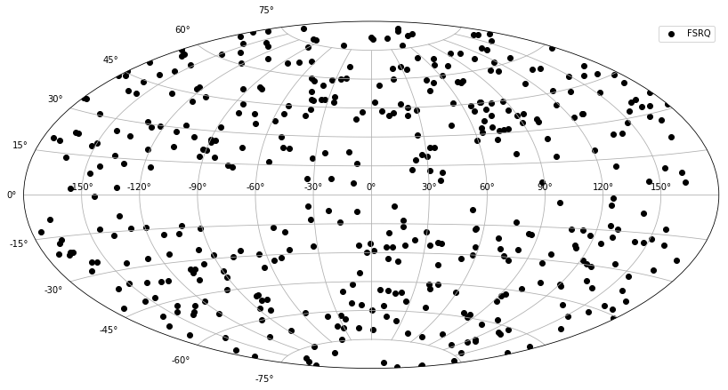
Selections in a Table
Here we select Sources according to their class and do some whole sky chart
In [24]:
# Get coordinates of FSRQs
fsrq = np.where( np.logical_or(table['CLASS1']=='fsrq ',table['CLASS1']=='FSQR '))
In [25]:
# This is here for plotting purpose...
#glon = glon.wrap_at(180*u.degree)

# Open figure
fig = plt.figure(figsize=(14,8))
ax = fig.add_subplot(111, projection="aitoff")
ax.scatter(coord[fsrq].l.wrap_at(180*u.degree).radian,
           coord[fsrq].b.radian,
           color = 'k', label='FSRQ')
ax.grid(True)
ax.legend()
# ax.invert_xaxis()  -> This does not work for projections...
Out[25]:
<matplotlib.legend.Legend at 0x11081d780>
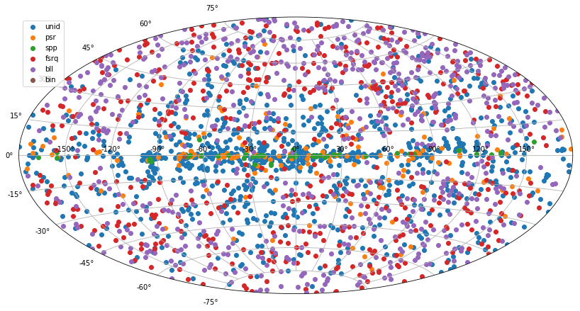
In [26]:
# Now do it for a series of classes
fig = plt.figure(figsize=(14,10))
ax = fig.add_subplot(111, projection="aitoff")

source_classes = ['','psr','spp', 'fsrq', 'bll', 'bin']

for source_class in source_classes:
    # We select elements with correct class in upper or lower characters
    index = np.array([_.strip().lower() == source_class for _ in table['CLASS1']])

    label = source_class if source_class else 'unid'

    ax.scatter(
        coord[index].l.wrap_at(180*u.degree).radian,
        coord[index].b.radian,
        label=label,
    )

ax.grid(True)
ax.legend()
Out[26]:
<matplotlib.legend.Legend at 0x10b5cecc0>
Creating tables
A Table is basically a dict mapping column names to column values,
where a column value is a Numpy array (or Quantity object, which is a
Numpy array sub-class). This implies that adding columns to a table
after creation is nice and easy, but adding a row is hard and slow,
basically all data has to be copied and all objects that make up a Table
have to be re-created.
Here’s one way to create a Table from scratch: put the data into a
list of dicts, and then call the Table constructor with the rows
option.
In [27]:
rows = [
    dict(a=42, b='spam'),
    dict(a=43, b='ham'),
]
my_table = Table(rows=rows)
my_table
Out[27]:
| a | b |
|---|---|
| int64 | str4 |
| 42 | spam |
| 43 | ham |
Writing tables
Writing tables to files is easy, you can just give the filename and
format you want. If you run a script repeatedly you might want to add
overwrite=True.
In [28]:
# Examples how to write a table in different formats
# Uncomment if you really want to do it

# my_table.write('/tmp/table.fits', format='fits')
# my_table.write('/tmp/table.fits.gz', format='fits')
# my_table.write('/tmp/table.ecsv', format='ascii.ecsv')
FITS (and some other formats, e.g. HDF5) support writing multiple tables
to a single file. The table.write API doesn’t support that directly
yet. Here’s how you can currently write multiple tables to a FITS file:
you have to convert the astropy.table.Table objects to
astropy.io.fits.BinTable objects, and then store them in a
astropy.io.fits.HDUList objects and call HDUList.writeto.
In [29]:
my_table2 = Table(data=dict(a=[1, 2, 3]))
hdu_list = fits.HDUList([
    fits.PrimaryHDU(), # need an empty primary HDU
    fits.table_to_hdu(my_table),
    fits.table_to_hdu(my_table2),
])
# hdu_list.writeto('tables.fits')
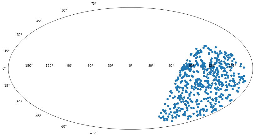
Using regions
Let’s try to find sources inside a circular region in the sky.
For this we will rely on the region package
We first create a circular region centered on a given SkyCoord with a given radius.
In [30]:
from regions import CircleSkyRegion

#center = SkyCoord.from_name("M31")
center = SkyCoord(ra='0h42m44.31s', dec='41d16m09.4s')

circle_region = CircleSkyRegion(
    center=center,
    radius=Angle(50, 'deg')
)
We now use the contains method to search objects in this circular region in the sky.
In [31]:
in_region = circle_region.contains(coord)
In [32]:
fig = plt.figure(figsize=(14,10))
ax = fig.add_subplot(111, projection="aitoff")
ax.scatter(coord[in_region].l.radian, coord[in_region].b.radian)
Out[32]:
<matplotlib.collections.PathCollection at 0x10b4c7a20>
Tables and pandas
pandas is one of the most-used packages
in the scientific Python stack. Numpy provides the ndarray object
and functions that operate on ndarray objects. Pandas provides the
Dataframe and Series objects, which roughly correspond to the
Astropy Table and Column objects. While both
pandas.Dataframe and astropy.table.Table can often be used to
work with tabular data, each has features that the other doesn’t. When
Astropy was started, it was decided to not base it on
pandas.Dataframe, but to introduce Table, mainly because
pandas.Dataframe doesn’t support multi-dimensional columns, but FITS
does and astronomers use sometimes.
But pandas.Dataframe has a ton of features that Table doesn’t,
and is highly optimised, so if you find something to be hard with
Table, you can convert it to a Dataframe and do your work there.
As explained in the interfacing with the pandas
package page in
the Astropy docs, it is easy to go back and forth between Table and
Dataframe:
table = Table.from_pandas(dataframe)
dataframe = table.to_pandas()
Let’s try it out with the Fermi-LAT catalog.
One little trick is needed when converting to a dataframe: we need to drop the multi-dimensional columns that the 3FGL catalog uses for a few columns (flux up/down errors, and lightcurves):
In [33]:
scalar_colnames = tuple(name for name in table.colnames if len(table[name].shape) <= 1)
data_frame = table[scalar_colnames].to_pandas()
In [34]:
# If you want to have a quick-look at the dataframe:
# data_frame
# data_frame.info()
# data_frame.describe()
In [35]:
# Just do demonstrate one of the useful DataFrame methods,
# this is how you can count the number of sources in each class:
data_frame['CLASS1'].value_counts()
Out[35]:
1010
bll       642
bcu       568
fsrq      446
PSR       143
spp        49
FSRQ       38
psr        24
BLL        18
glc        15
rdg        12
SNR        12
snr        11
PWN        10
BCU         5
sbg         4
agn         3
nlsy1       3
ssrq        3
HMB         3
RDG         3
GAL         2
NLSY1       2
pwn         2
gal         1
sey         1
BIN         1
NOV         1
css         1
SFR         1
Name: CLASS1, dtype: int64
If you’d like to learn more about pandas, have a look here or here.
Exercises
- When searched for the hardest and softest sources in 3FGL we did not look at the type of spectrum (PL, ECPL etc), find the hardest and softest PL sources instead.
- Replot the full sky chart of sources in ra-dec instead of galactic coordinates
- Find the 3FGL sources visible from Paris now