This is a fixed-text formatted version of a Jupyter notebook.
You can contribute with your own notebooks in this GitHub repository.
Source files: cta_simulation.ipynb | cta_simulation.py
CTA simulation tools
Introduction
In this tutorial we will simulate the expected counts of a Fermi/LAT source in the CTA energy range.
We will go through the following topics:
- handling of Fermi/LAT 3FHL catalogue with gammapy.catalog.SourceCatalog3FHL
- handling of EBL tables with gammapy.spectrum.TableModel
- handling of CTA responses with gammapy.scripts.CTAPerf
- simulation of an observation for a given set of parameters with gammapy.scripts.CTAObservationSimulation
- Illustration of Sherpa power to fit an observation with a user model (coming soon)
Setup
In order to deal with plots we will begin with matplotlib import:
In [1]:
%matplotlib inline
import matplotlib.pyplot as plt
PKS 2155-304 selection from the 3FHL Fermi/LAT catalogue
We will start by selecting the source PKS 2155-304 in the 3FHL Fermi/LAT catalogue for further use.
In [2]:
from gammapy.catalog import SourceCatalog3FHL

# load catalogs
fermi_3fhl = SourceCatalog3FHL()
name = 'PKS 2155-304'
source = fermi_3fhl[name]
We can then access the caracteristics of the source via the data
attribut and select its spectral model for further use.
In [3]:
redshift = source.data['Redshift']
src_spectral_model = source.spectral_model
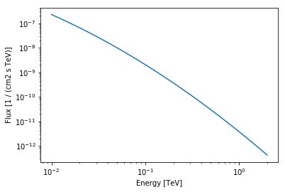
Here is an example on how to plot the source spectra
In [4]:
# plot the Fermi/LAT model
import astropy.units as u
src_spectral_model.plot(energy_range=[10 * u.GeV, 2 *u.TeV])
Out[4]:
<matplotlib.axes._subplots.AxesSubplot at 0x11332ec88>
Select a model for EBL absorption
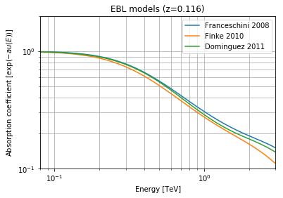
We will need to modelise EBL (extragalactic background light) attenuation to have get a ‘realistic’ simulation. Different models are available in GammaPy. Here is an example on how to deal with the absorption coefficients.
In [5]:
from gammapy.spectrum.models import Absorption

# Load models for PKS 2155-304 redshift
dominguez = Absorption.read_builtin('dominguez').table_model(redshift)
franceschini = Absorption.read_builtin('franceschini').table_model(redshift)
finke = Absorption.read_builtin('finke').table_model(redshift)
From here you can have access to the absorption coefficient for a given energy.
In [6]:
energy = 1 * u.TeV
abs_value = dominguez.evaluate(energy=energy, scale=1)
print('absorption({} {}) = {}'.format(energy.value, energy.unit, abs_value))
absorption(1.0 TeV) = 0.2877190694779645
Below is an example to plot EBL absorption for different models
In [7]:
# start customised plot
energy_range = [0.08, 3] * u.TeV
ax = plt.gca()
opts = dict(energy_range=energy_range, energy_unit='TeV', ax=ax)
franceschini.plot(label='Franceschini 2008', **opts)
finke.plot(label='Finke 2010', **opts)
dominguez.plot(label='Dominguez 2011', **opts)

# tune plot
ax.set_ylabel(r'Absorption coefficient [$\exp{(-        au(E))}$]')
ax.set_xlim(energy_range.value)  # we get ride of units
ax.set_ylim([1.e-1, 2.])
ax.set_yscale('log')
ax.set_title('EBL models (z=' + str(redshift) + ')')
plt.grid(which='both')
plt.legend(loc='best') # legend

# show plot
plt.show()
CTA instrument response functions
Here we are going to deal with CTA point-like instrument response functions (public version, production 2). Data format for point-like IRF is still missing. For now, a lot of efforts is made to define full-containment IRFs (https://gamma-astro-data-formats.readthedocs.io/en/latest/irfs/index.html). In the meantime a temporary format is used in gammapy. It will evolved.
To simulate one observation we need the following IRFs: - effective area as a function of true energy (energy-dependent theta square cute) - background rate as a function of reconstructed energy (energy-dependent theta square cute) - migration matrix, e_reco/e_true as a function of true energy
To handle CTA’s responses we will use the CTAPerf class
In [8]:
from gammapy.scripts import CTAPerf
# South array optimisation for faint source
filename = '$GAMMAPY_EXTRA/datasets/cta/perf_prod2/point_like_non_smoothed/South_50h.fits.gz'
cta_perf = CTAPerf.read(filename)
cta_perf.peek()
---------------------------------------------------------------------------
AttributeError                            Traceback (most recent call last)
/opt/local/Library/Frameworks/Python.framework/Versions/3.6/lib/python3.6/site-packages/IPython/core/formatters.py in __call__(self, obj)
    339                 pass
    340             else:
--> 341                 return printer(obj)
    342             # Finally look for special method names
    343             method = get_real_method(obj, self.print_method)

/opt/local/Library/Frameworks/Python.framework/Versions/3.6/lib/python3.6/site-packages/IPython/core/pylabtools.py in <lambda>(fig)
    236
    237     if 'png' in formats:
--> 238         png_formatter.for_type(Figure, lambda fig: print_figure(fig, 'png', **kwargs))
    239     if 'retina' in formats or 'png2x' in formats:
    240         png_formatter.for_type(Figure, lambda fig: retina_figure(fig, **kwargs))

/opt/local/Library/Frameworks/Python.framework/Versions/3.6/lib/python3.6/site-packages/IPython/core/pylabtools.py in print_figure(fig, fmt, bbox_inches, **kwargs)
    120
    121     bytes_io = BytesIO()
--> 122     fig.canvas.print_figure(bytes_io, **kw)
    123     data = bytes_io.getvalue()
    124     if fmt == 'svg':

/opt/local/Library/Frameworks/Python.framework/Versions/3.6/lib/python3.6/site-packages/matplotlib/backend_bases.py in print_figure(self, filename, dpi, facecolor, edgecolor, orientation, format, **kwargs)
   2206                     orientation=orientation,
   2207                     dryrun=True,
-> 2208                     **kwargs)
   2209                 renderer = self.figure._cachedRenderer
   2210                 bbox_inches = self.figure.get_tightbbox(renderer)

/opt/local/Library/Frameworks/Python.framework/Versions/3.6/lib/python3.6/site-packages/matplotlib/backends/backend_agg.py in print_png(self, filename_or_obj, *args, **kwargs)
    505
    506     def print_png(self, filename_or_obj, *args, **kwargs):
--> 507         FigureCanvasAgg.draw(self)
    508         renderer = self.get_renderer()
    509         original_dpi = renderer.dpi

/opt/local/Library/Frameworks/Python.framework/Versions/3.6/lib/python3.6/site-packages/matplotlib/backends/backend_agg.py in draw(self)
    428             if toolbar:
    429                 toolbar.set_cursor(cursors.WAIT)
--> 430             self.figure.draw(self.renderer)
    431         finally:
    432             if toolbar:

/opt/local/Library/Frameworks/Python.framework/Versions/3.6/lib/python3.6/site-packages/matplotlib/artist.py in draw_wrapper(artist, renderer, *args, **kwargs)
     53                 renderer.start_filter()
     54
---> 55             return draw(artist, renderer, *args, **kwargs)
     56         finally:
     57             if artist.get_agg_filter() is not None:

/opt/local/Library/Frameworks/Python.framework/Versions/3.6/lib/python3.6/site-packages/matplotlib/figure.py in draw(self, renderer)
   1293
   1294             mimage._draw_list_compositing_images(
-> 1295                 renderer, self, artists, self.suppressComposite)
   1296
   1297             renderer.close_group('figure')

/opt/local/Library/Frameworks/Python.framework/Versions/3.6/lib/python3.6/site-packages/matplotlib/image.py in _draw_list_compositing_images(renderer, parent, artists, suppress_composite)
    136     if not_composite or not has_images:
    137         for a in artists:
--> 138             a.draw(renderer)
    139     else:
    140         # Composite any adjacent images together

/opt/local/Library/Frameworks/Python.framework/Versions/3.6/lib/python3.6/site-packages/matplotlib/artist.py in draw_wrapper(artist, renderer, *args, **kwargs)
     53                 renderer.start_filter()
     54
---> 55             return draw(artist, renderer, *args, **kwargs)
     56         finally:
     57             if artist.get_agg_filter() is not None:

/opt/local/Library/Frameworks/Python.framework/Versions/3.6/lib/python3.6/site-packages/matplotlib/axes/_base.py in draw(self, renderer, inframe)
   2397             renderer.stop_rasterizing()
   2398
-> 2399         mimage._draw_list_compositing_images(renderer, self, artists)
   2400
   2401         renderer.close_group('axes')

/opt/local/Library/Frameworks/Python.framework/Versions/3.6/lib/python3.6/site-packages/matplotlib/image.py in _draw_list_compositing_images(renderer, parent, artists, suppress_composite)
    136     if not_composite or not has_images:
    137         for a in artists:
--> 138             a.draw(renderer)
    139     else:
    140         # Composite any adjacent images together

/opt/local/Library/Frameworks/Python.framework/Versions/3.6/lib/python3.6/site-packages/matplotlib/artist.py in draw_wrapper(artist, renderer, *args, **kwargs)
     53                 renderer.start_filter()
     54
---> 55             return draw(artist, renderer, *args, **kwargs)
     56         finally:
     57             if artist.get_agg_filter() is not None:

/opt/local/Library/Frameworks/Python.framework/Versions/3.6/lib/python3.6/site-packages/matplotlib/collections.py in draw(self, renderer)
   1871                 offsets = np.column_stack([xs, ys])
   1872
-> 1873         self.update_scalarmappable()
   1874
   1875         if not transform.is_affine:

/opt/local/Library/Frameworks/Python.framework/Versions/3.6/lib/python3.6/site-packages/matplotlib/collections.py in update_scalarmappable(self)
    740             return
    741         if self._is_filled:
--> 742             self._facecolors = self.to_rgba(self._A, self._alpha)
    743         elif self._is_stroked:
    744             self._edgecolors = self.to_rgba(self._A, self._alpha)

/opt/local/Library/Frameworks/Python.framework/Versions/3.6/lib/python3.6/site-packages/matplotlib/cm.py in to_rgba(self, x, alpha, bytes, norm)
    273         x = ma.asarray(x)
    274         if norm:
--> 275             x = self.norm(x)
    276         rgba = self.cmap(x, alpha=alpha, bytes=bytes)
    277         return rgba

/opt/local/Library/Frameworks/Python.framework/Versions/3.6/lib/python3.6/site-packages/matplotlib/colors.py in __call__(self, value, clip)
   1198             resdat -= vmin
   1199             np.power(resdat, gamma, resdat)
-> 1200             resdat /= (vmax - vmin) ** gamma
   1201
   1202             result = np.ma.array(resdat, mask=result.mask, copy=False)

~/Library/Python/3.6/lib/python/site-packages/astropy/units/quantity.py in __array_ufunc__(self, function, method, *inputs, **kwargs)
    641             return result
    642
--> 643         return self._result_as_quantity(result, unit, out)
    644
    645     def _result_as_quantity(self, result, unit, out):

~/Library/Python/3.6/lib/python/site-packages/astropy/units/quantity.py in _result_as_quantity(self, result, unit, out)
    680         # the output is of the correct Quantity subclass, as it was passed
    681         # through check_output.
--> 682         out._set_unit(unit)
    683         return out
    684

AttributeError: 'numpy.ndarray' object has no attribute '_set_unit'
<matplotlib.figure.Figure at 0x11354e9e8>
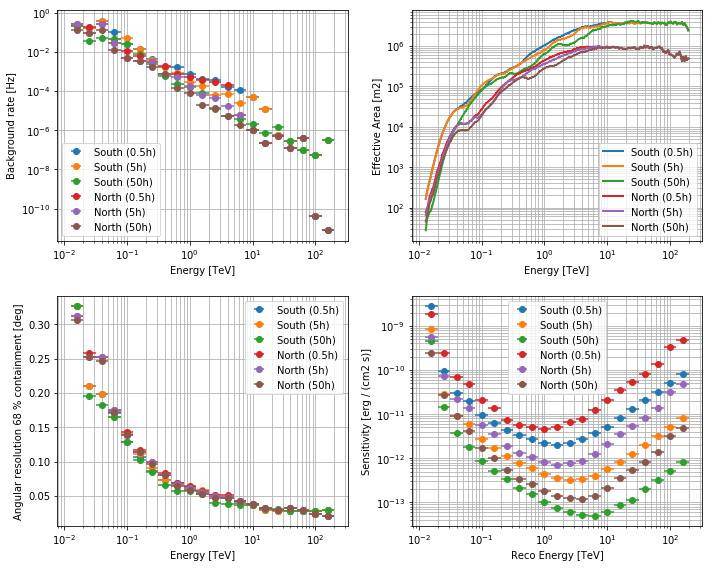
Different optimisations are available for different type of source (bright, 0.5h; medium, 5h; faint, 50h). Here is an example to have a quick look to the different optimisation
In [9]:
prod_dir = '$GAMMAPY_EXTRA/datasets/cta/perf_prod2/point_like_non_smoothed/'
opti = ['0.5h', '5h', '50h']
site = ['South', 'North']
cta_perf_list = []  # will be filled with different performance
labels = []  # will be filled with different performance labels for the legend
for isite in site:
    for iopti in opti:
        filename = prod_dir + '/' + isite + '_' + iopti + '.fits.gz'
        cta_perf = CTAPerf.read(filename)
        cta_perf_list.append(cta_perf)
        labels.append(isite + ' (' + iopti + ')')

CTAPerf.superpose_perf(cta_perf_list, labels)
CTA simulation of an observation
Now we are going to simulate the expected counts in the CTA energy range. To do so we will need to specify a target (caracteristics of the source) and the parameters of the observation (such as time, ON/OFF normalisation, etc.)
Target definition
In [10]:
# define target spectral model absorbed by EBL
from gammapy.spectrum.models import Absorption, AbsorbedSpectralModel

absorption = Absorption.read_builtin('dominguez')
spectral_model = AbsorbedSpectralModel(
    spectral_model=src_spectral_model,
    absorption=absorption,
    parameter=redshift,
)
# define target
from gammapy.scripts.cta_utils import Target
target = Target(
    name=source.data['Source_Name'],  # from the 3FGL catalogue source class
    model=source.spectral_model,  # defined above
)
print(target)
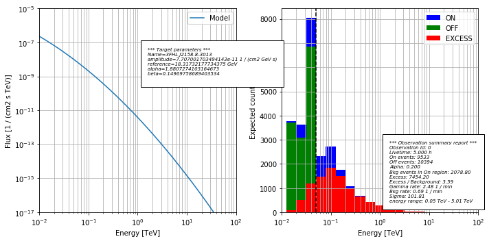
*** Target parameters ***
Name=3FHL J2158.8-3013
amplitude=7.707001703494143e-11 1 / (cm2 GeV s)
reference=18.31732177734375 GeV
alpha=1.8807274103164673
beta=0.14969758689403534
Observation definition
In [11]:
from gammapy.scripts.cta_utils import ObservationParameters
alpha = 0.2 * u.Unit('')  # normalisation between ON and OFF regions
livetime = 5. * u.h
# energy range used for statistics (excess, significance, etc.)
emin, emax = 0.05 * u.TeV, 5 * u.TeV
params = ObservationParameters(
    alpha=alpha, livetime=livetime,
    emin=emin, emax=emax,
)
print(params)
*** Observation parameters summary ***
alpha=0.2 []
livetime=5.0 [h]
emin=0.05 [TeV]
emax=5.0 [TeV]
Performance
In [12]:
from gammapy.scripts import CTAPerf
# PKS 2155-304 is 10 % of Crab at 1 TeV ==> intermediate source
filename = '$GAMMAPY_EXTRA/datasets/cta/perf_prod2/point_like_non_smoothed/South_5h.fits.gz'
perf = CTAPerf.read(filename)
Simulation
Here we are going to simulate what we expect to see with CTA and measure the duration of the simulation
In [13]:
from gammapy.scripts.cta_utils import CTAObservationSimulation

simu = CTAObservationSimulation.simulate_obs(
    perf=perf,
    target=target,
    obs_param=params,
)

# print simulation results
print(simu)
*** Observation summary report ***
Observation Id: 0
Livetime: 5.000 h
On events: 9533
Off events: 10394
Alpha: 0.200
Bkg events in On region: 2078.80
Excess: 7454.20
Excess / Background: 3.59
Gamma rate: 2.48 1 / min
Bkg rate: 0.69 1 / min
Sigma: 101.81
energy range: 0.05 TeV - 5.01 TeV
Now we can take a look at the excess, ON and OFF distributions
In [14]:
CTAObservationSimulation.plot_simu(simu, target)
We can access simulation parameters via the gammapy.spectrum.SpectrumStats attribute of the gammapy.spectrum.SpectrumObservation class:
In [15]:
stats = simu.total_stats_safe_range
stats_dict = stats.to_dict()
print('excess: {}'.format(stats_dict['excess']))
print('sigma: {:.1f}'.format(stats_dict['sigma']))
excess: 7454.2
sigma: 101.8
Finally, you can get statistics for every reconstructed energy bin with:
In [16]:
table = simu.stats_table()
# Here we only print part of the data from the table
table[['energy_min', 'energy_max', 'excess', 'background', 'sigma']][:10]
Out[16]:
| energy_min | energy_max | excess | background | sigma |
|---|---|---|---|---|
| TeV | TeV | |||
| float64 | float64 | float64 | float64 | float64 |
| 0.012589254416525364 | 0.019952623173594475 | 80.2 | 3698.8 | 1.19876696834 |
| 0.019952623173594475 | 0.03162277862429619 | 523.2 | 3101.8 | 8.31247160578 |
| 0.03162277862429619 | 0.05011872574687004 | 1179.8 | 6852.2 | 12.6036218473 |
| 0.05011872574687004 | 0.07943282276391983 | 1486.4 | 827.6 | 37.1420674171 |
| 0.07943282276391983 | 0.1258925497531891 | 1845.2 | 884.8 | 43.4004197611 |
| 0.1258925497531891 | 0.19952623546123505 | 1510.6 | 235.4 | 52.3960324108 |
| 0.19952623546123505 | 0.3162277638912201 | 1004.0 | 73.0 | 48.5896826006 |
| 0.3162277638912201 | 0.5011872053146362 | 644.4 | 32.6 | 40.7290245347 |
| 0.5011872053146362 | 0.7943282127380371 | 421.8 | 12.2 | 34.7549641246 |
| 0.7943282127380371 | 1.258925437927246 | 273.2 | 4.8 | 28.9374446728 |
Exercises
- do the same thing for the source 1ES 2322-40.9 (faint BL Lac object)
- repeat the procedure 10 times and average detection results (excess and significance)
- estimate the time needed to have a 5-sigma detection for Cen A (core)