This is a fixed-text formatted version of a Jupyter notebook.
You can contribute with your own notebooks in this GitHub repository.
Source files: data_fermi_lat.ipynb | data_fermi_lat.py
Fermi-LAT data with Gammapy
Introduction
This tutorial will show you how to work with pepared Fermi-LAT datasets.
The main class to load and handle the data is:
Additionally we will use objects of these types:
- gammapy.data.EventList for event lists.
- gammapy.irf.EnergyDependentTablePSF for the point spread function.
- gammapy.cube.SkyCube for the galactic diffuse background model.
- gammapy.cube.SkyCubeHPX for the exposure.
- gammapy.spectrum.models.TableModel for the isotropic diffuse model.
- gammapy.image.FermiLATBasicImageEstimator for generating a full WCS dataset, that can be used as an input for image based analyses.
Setup
IMPORTANT: For this notebook you have to get the prepared datasets provided in the gammapy-fermi-lat-data repository. Please follow the instructions here to download the data and setup your environment.
In [1]:
%matplotlib inline
import numpy as np
import matplotlib.pyplot as plt
In [2]:
from astropy import units as u
from astropy.visualization import simple_norm
from gammapy.datasets import FermiLATDataset
from gammapy.image import SkyImage, FermiLATBasicImageEstimator
FermiLATDataset class
To access the prepared Fermi-LAT datasets Gammapy provides a convenience class called FermiLATDataset. It is initialized with a path to an index configuration file, which tells the dataset class where to find the data. Once the object is initialized the data can be accessed as properties of this object, which return the corresponding Gammapy data objects for event lists, sky images and point spread functions (PSF).
So let’s start with exploring the Fermi-LAT 2FHL dataset:
In [3]:
# initialize dataset
dataset = FermiLATDataset('$GAMMAPY_FERMI_LAT_DATA/2fhl/fermi_2fhl_data_config.yaml')
print(dataset)
Fermi-LAT 2FHL dataset
======================
Filenames:
  counts  : fermi_2fhl_counts_cube_hpx.fits.gz
  events  : fermi_2fhl_events.fits.gz
  exposure: fermi_2fhl_exposure_cube_hpx.fits.gz
  isodiff : ../isodiff/iso_P8R2_SOURCE_V6_v06.txt
  livetime: fermi_2fhl_livetime_cube.fits.gz
  psf     : fermi_2fhl_psf_gc.fits.gz
Events
The first data member we will inspect in more detail is the event list.
It can be accessed by the dataset.events property and returns an
instance of the Gammapy
gammapy.data.EventList
class:
In [4]:
# access events data member
events = dataset.events
print(events)
EventList info:
- Number of events: 60275
- Median energy: 80340.5078125 MeV
The full event data is available via the EventList.table property,
which returns an
astropy.table.Table
instance. In case of the Fermi-LAT event list this contains all the
additional information on positon, zenith angle, earth azimuth angle,
event class, event type etc. Execute the following cell to take a look
at the event list table:
In [5]:
events.table
Out[5]:
| ENERGY | RA | DEC | L | B | THETA | PHI | ZENITH_ANGLE | EARTH_AZIMUTH_ANGLE | TIME | EVENT_ID | RUN_ID | RECON_VERSION | CALIB_VERSION [3] | EVENT_CLASS [32] | EVENT_TYPE [32] | CONVERSION_TYPE | LIVETIME | DIFRSP0 | DIFRSP1 | DIFRSP2 | DIFRSP3 | DIFRSP4 |
|---|---|---|---|---|---|---|---|---|---|---|---|---|---|---|---|---|---|---|---|---|---|---|
| MeV | deg | deg | deg | deg | deg | deg | deg | deg | s | s | ||||||||||||
| float32 | float32 | float32 | float32 | float32 | float32 | float32 | float32 | float32 | float64 | int32 | int32 | int16 | int16 | bool | bool | int16 | float64 | float32 | float32 | float32 | float32 | float32 |
| 145927.0 | 291.662 | 42.2341 | 74.5437 | 11.8678 | 38.0455 | 83.5358 | 55.6387 | 314.034 | 239561457.866 | 4851437 | 239559565 | 0 | 0 .. 0 | False .. True | False .. True | 0 | 275.698088974 | 0.0 | 0.0 | 0.0 | 0.0 | 0.0 |
| 221273.0 | 46.9858 | -40.6389 | 247.489 | -58.8739 | 34.1051 | 224.209 | 68.2524 | 198.319 | 239562739.085 | 7521432 | 239559565 | 0 | 0 .. 0 | False .. True | False .. True | 0 | 64.7974931598 | 0.0 | 0.0 | 0.0 | 0.0 | 0.0 |
| 57709.2 | 121.841 | 49.2288 | 169.868 | 32.3017 | 71.5636 | 34.2925 | 36.7173 | 25.5439 | 239563180.302 | 8690693 | 239559565 | 0 | 0 .. 0 | False .. True | False .. True | 0 | 30.57218647 | 0.0 | 0.0 | 0.0 | 0.0 | 0.0 |
| 221224.0 | 83.5626 | -4.21744 | 207.783 | -19.0771 | 20.5089 | 92.1605 | 32.3033 | 239.141 | 239563382.213 | 9208424 | 239559565 | 0 | 0 .. 0 | False .. True | False .. True | 0 | 27.4125095904 | 0.0 | 0.0 | 0.0 | 0.0 | 0.0 |
| 698997.0 | 320.895 | -1.32789 | 51.2218 | -33.9718 | 35.3621 | 158.741 | 12.0867 | 72.2029 | 239566572.951 | 2480483 | 239565645 | 0 | 0 .. 0 | False .. True | False .. True | 0 | 106.475481123 | 0.0 | 0.0 | 0.0 | 0.0 | 0.0 |
| 119159.0 | 318.811 | 12.3028 | 62.6361 | -24.416 | 26.5896 | 213.894 | 17.7156 | 23.9409 | 239572348.06 | 1725276 | 239571670 | 0 | 0 .. 0 | False .. True | False .. True | 0 | 185.346427292 | 0.0 | 0.0 | 0.0 | 0.0 | 0.0 |
| 56175.6 | 279.251 | 47.8835 | 76.6915 | 22.0739 | 29.1034 | 61.0048 | 62.1731 | 321.104 | 239572763.431 | 76017 | 239572736 | 0 | 0 .. 0 | False .. True | False .. True | 0 | 24.4507339597 | 0.0 | 0.0 | 0.0 | 0.0 | 0.0 |
| 1.41812e+06 | 100.311 | -47.4481 | 256.468 | -21.2641 | 61.2256 | 294.18 | 90.4753 | 144.149 | 239573788.813 | 1781569 | 239572736 | 0 | 0 .. 0 | False .. True | False .. True | 0 | 68.271614641 | 0.0 | 0.0 | 0.0 | 0.0 | 0.0 |
| 62164.9 | 331.492 | -41.2264 | 359.42 | -53.4049 | 28.1408 | 229.927 | 52.0142 | 189.054 | 239578601.168 | 2000700 | 239577663 | 0 | 0 .. 0 | False .. True | False .. True | 0 | 90.332262665 | 0.0 | 0.0 | 0.0 | 0.0 | 0.0 |
| ... | ... | ... | ... | ... | ... | ... | ... | ... | ... | ... | ... | ... | ... | ... | ... | ... | ... | ... | ... | ... | ... | ... |
| 51296.8 | 79.0311 | 78.9327 | 133.868 | 22.2399 | 51.1726 | 267.814 | 99.7602 | 357.79 | 444418973.822 | 1284853 | 444418590 | 0 | 0 .. 0 | False .. True | False .. True | 0 | 181.6889835 | 0.0 | 0.0 | 0.0 | 0.0 | 0.0 |
| 60315.7 | 243.681 | -50.5669 | 332.43 | 0.28268 | 24.8501 | 255.683 | 74.8804 | 195.14 | 444421777.761 | 6582949 | 444418590 | 0 | 0 .. 0 | False .. True | False .. False | 1 | 57.3358902931 | 0.0 | 0.0 | 0.0 | 0.0 | 0.0 |
| 90000.1 | 282.698 | -33.1987 | 2.66219 | -14.3339 | 8.49144 | 343.559 | 47.3965 | 191.033 | 444422182.738 | 7507466 | 444418590 | 0 | 0 .. 0 | False .. True | False .. True | 0 | 187.602469146 | 0.0 | 0.0 | 0.0 | 0.0 | 0.0 |
| 61988.7 | 247.98 | -48.1091 | 336.146 | 0.0220339 | 33.6499 | 144.271 | 80.3966 | 221.396 | 444422758.145 | 8699147 | 444418590 | 0 | 0 .. 0 | False .. True | False .. True | 0 | 39.2098327279 | 0.0 | 0.0 | 0.0 | 0.0 | 0.0 |
| 54282.9 | 159.924 | -58.3628 | 286.362 | 0.205554 | 24.1196 | 287.138 | 65.0847 | 177.524 | 444425794.794 | 2522237 | 444424619 | 0 | 0 .. 0 | False .. True | False .. True | 0 | 196.209668875 | 0.0 | 0.0 | 0.0 | 0.0 | 0.0 |
| 146728.0 | 244.848 | -46.5876 | 335.754 | 2.60326 | 45.2539 | 5.33644 | 91.871 | 137.032 | 444425911.819 | 2705210 | 444424619 | 0 | 0 .. 0 | False .. True | False .. False | 1 | 65.6327857375 | 0.0 | 0.0 | 0.0 | 0.0 | 0.0 |
| 135433.0 | 83.5278 | 27.9053 | 179.529 | -2.69106 | 17.4911 | 52.0858 | 53.306 | 313.822 | 444430968.968 | 939188 | 444430599 | 0 | 0 .. 0 | False .. True | False .. False | 1 | 97.6446831226 | 0.0 | 0.0 | 0.0 | 0.0 | 0.0 |
| 61592.1 | 231.214 | -5.45521 | 357.435 | 40.6473 | 46.6356 | 141.047 | 62.7584 | 256.631 | 444433607.906 | 5443944 | 444430599 | 0 | 0 .. 0 | False .. True | False .. False | 1 | 28.7290657759 | 0.0 | 0.0 | 0.0 | 0.0 | 0.0 |
| 80480.8 | 228.244 | -45.044 | 327.561 | 10.9528 | 37.3149 | 193.714 | 83.3882 | 221.57 | 444433702.069 | 5612443 | 444430599 | 0 | 0 .. 0 | False .. True | False .. False | 1 | 122.891819298 | 0.0 | 0.0 | 0.0 | 0.0 | 0.0 |
| 124449.0 | 238.008 | -51.0371 | 329.429 | 2.3006 | 32.4522 | 199.504 | 80.9768 | 214.48 | 444433764.433 | 5723361 | 444430599 | 0 | 0 .. 0 | False .. True | False .. True | 0 | 185.255487204 | 0.0 | 0.0 | 0.0 | 0.0 | 0.0 |
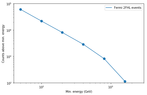
As a short analysis example we will count the number of events above a certain minimum energy:
In [6]:
# define energy thresholds
energies = [50, 100, 200, 400, 800, 1600] * u.GeV

n_events_above_energy = []

for energy in energies:
    n = (events.energy > energy).sum()
    n_events_above_energy.append(n)
    print("Number of events above {0:4.0f}: {1:5.0f}".format(energy, n))
Number of events above   50 GeV: 60275
Number of events above  100 GeV: 21874
Number of events above  200 GeV:  8028
Number of events above  400 GeV:  2884
Number of events above  800 GeV:   821
Number of events above 1600 GeV:   113
And plot it against energy:
In [7]:
plt.figure(figsize=(8, 5))
events_plot = plt.plot(energies.value, n_events_above_energy, label='Fermi 2FHL events')
plt.scatter(energies.value, n_events_above_energy, s=60, c=events_plot[0].get_color())
plt.loglog()
plt.xlabel("Min. energy (GeV)")
plt.ylabel("Counts above min. energy")
plt.xlim(4E1, 3E3)
plt.ylim(1E2, 1E5)
plt.legend()
Out[7]:
<matplotlib.legend.Legend at 0x113e3cb38>
PSF
Next we will tke a closer look at the PSF. The dataset contains a
precomputed PSF model for one position of the sky (in this case the
Galactic center). It can be accessed by the dataset.psf property and
returns an instance of the Gammapy
gammapy.irf.EnergyDependentTablePSF
class:
In [8]:
psf = dataset.psf
print(psf)
EnergyDependentTablePSF
-----------------------

Axis info:
  offset         : size =   300, min =  0.000 deg, max =  9.933 deg
  energy         : size =    17, min = 50.000 GeV, max = 2000.000 GeV
  exposure       : size =    17, min = 184244434125.149 cm2 s, max = 308160738535.443 cm2 s

Containment info:
  68.0% containment radius at  10 GeV: 0.10 deg
  68.0% containment radius at 100 GeV: 0.10 deg
  95.0% containment radius at  10 GeV: 0.52 deg
  95.0% containment radius at 100 GeV: 0.43 deg
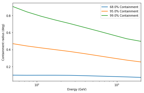
To get an idea of the size of the PSF we check how the containment radii of the Fermi-LAT PSF vari with energy and different containment fractions:
In [9]:
plt.figure(figsize=(8, 5))
psf.plot_containment_vs_energy(linewidth=2, fractions=[0.68, 0.95, 0.99])
plt.xlim(50, 2000)
plt.show()
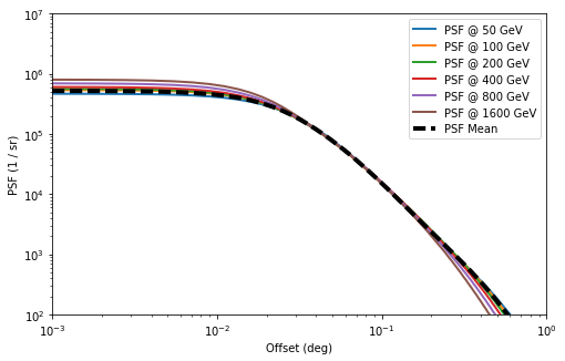
In addition we can check how the actual shape of the PSF varies with energy and compare it against the mean PSF between 50 GeV and 2000 GeV:
In [10]:
plt.figure(figsize=(8, 5))

for energy in energies:
    psf_at_energy = psf.table_psf_at_energy(energy)
    psf_at_energy.plot_psf_vs_theta(label='PSF @ {:.0f}'.format(energy), lw=2)

erange = [50, 2000] * u.GeV
psf_mean = psf.table_psf_in_energy_band(energy_band=erange, spectral_index=2.3)
psf_mean.plot_psf_vs_theta(label='PSF Mean', lw=4, c="k", ls='--')

plt.xlim(1E-3, 1)
plt.ylim(1E2, 1E7)
plt.legend()
Out[10]:
<matplotlib.legend.Legend at 0x114256390>
Exposure
The Fermi-LAT datatset contains the energy-dependent exposure for the
whole sky stored using a HEALPIX pixelisation of the sphere. It can be
accessed by the dataset.exposure property and returns an instance of
the Gammapy gammapy.cube.SkyCubeHPX class:
In [11]:
exposure = dataset.exposure
print(exposure)
Healpix sky cube exposure with shape=(18, 12288) and unit=cm2 s:
 n_pix:    12288  coord_type:    galactic         coord_unit:    deg
 n_energy:    18  unit_energy: MeV
In [12]:
# define reference image using a cartesian projection
image_ref = SkyImage.empty(nxpix=360, nypix=180, binsz=1, proj='CAR')

# reproject HEALPIC sky cube
exposure_reprojected = exposure.reproject(image_ref)
In [13]:
exposure_reprojected.show()
Out[13]:
<function gammapy.cube.core.SkyCube.show.<locals>.show_image>
You can use the slider to slide through the different energy bands.
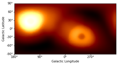
Galactic diffuse background
The Fermi-LAT collaboration provides a galactic diffuse emission model,
that can be used as a background model for Fermi-LAT data analysis.
Currently Gammapy only supports the latest model (gll_iem_v06.fits).
It can be accessed by the dataset.galactic_diffuse property and
returns an instance of the Gammapy
gammapy.cube.SkyCube
class:
In [14]:
galactic_diffuse = dataset.galactic_diffuse
print(galactic_diffuse)
Sky cube galactic diffuse with shape=(30, 1441, 2880) and unit=1 / (cm2 MeV s sr):
 n_lon:     2880  type_lon:    GLON-CAR         unit_lon:    deg
 n_lat:     1441  type_lat:    GLAT-CAR         unit_lat:    deg
 n_energy:    30  unit_energy: MeV
In [15]:
norm = simple_norm(image_ref.data, stretch='log', clip=True)
galactic_diffuse.show(norm=norm)
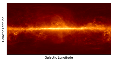
Out[15]:
<function gammapy.cube.core.SkyCube.show.<locals>.show_image>
Again you can use the slider to slide through the different energy bands. E.g. note how the Fermi-Bubbles become more present at higher energies (higher value of idx).
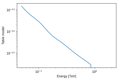
Isotropic diffuse background
Additionally to the galactic diffuse model, there is an isotropic
diffuse component. It can be accessed by the
dataset.isotropic_diffuse property and returns an instance of the
Gammapy
gammapy.spectrum.models.TableModel
class:
In [16]:
isotropic_diffuse = dataset.isotropic_diffuse
print(isotropic_diffuse)
TableModel
ParameterList
Parameter(name='amplitude', value=1, unit='', min=0, max=None, frozen=False)

Covariance: None
We can plot the model in the energy range between 50 GeV and 2000 GeV:
In [17]:
erange = [50, 2000] * u.GeV
isotropic_diffuse.plot(erange)
Out[17]:
<matplotlib.axes._subplots.AxesSubplot at 0x114e08be0>
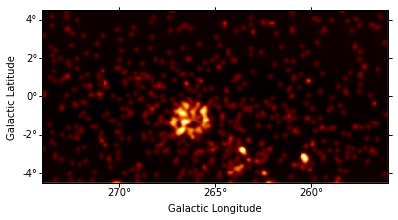
Estimating basic input sky images for high level analyses
Finally we’d like to use the prepared 2FHL dataset to generate a set of basic sky images, that a can be used as input for high level analyses, e.g. morphology fits, region based flux measurements, computation of significance images etc. For this purpose Gammapy provides a convenience class called gammapy.image.FermiLATBasicImageEstimator. First we define a reference image, that specifies the region we’d like to analyse. In this case we choose the Vela region.
In [18]:
image_ref = SkyImage.empty(
    nxpix=360, nypix=180,
    binsz=0.05,
    xref=265, yref=0,
)
Next we choose the energy range and initialize the
FermiLATBasicImageEstimator object:
In [19]:
emin, emax = [50, 2000] * u.GeV
image_estimator = FermiLATBasicImageEstimator(
    reference=image_ref,
    emin=emin, emax=emax,
)
Finally we run the image estimation by calling .run() and parsing
the dataset object:
In [20]:
images_basic = image_estimator.run(dataset)
The image estimator now computes a set of sky images for the reference
region and energy range we defined above. The result images_basic is
a
gammapy.image.SkyImageList
object containing the following images:
- counts: counts image containing the binned event list
- background: predicted number of background counts computed from the sum of the galactic and isotropic diffuse model, given the exposure.
- exposure: integrated exposure assuming a powerlaw with spectral index 2.3 in the given energy range
- excess: backround substracted counts image
- flux: measured flux, computed from excess divided by exposure
- psf: sky image of the exposure weighted mean PSF in the given energy range
You can check the contained images as following:
In [21]:
images_basic.names
Out[21]:
['counts', 'background', 'exposure', 'excess', 'flux', 'psf']
To check whether the image estimation was succesfull we’ll take a look at the flux image, smoothing it in advance with a Gaussian kernel of 0.2 deg:
In [22]:
smoothed_flux = images_basic['flux'].smooth(
    kernel='gauss', radius=0.2 * u.deg)
smoothed_flux.show()
Exercises
- Try to reproject the exposure using an
AITprojection. - Try to find the spectral index of the isotropic diffuse model using a
method off the
TableModelinstance. - Compute basic sky images for different regions (e.g. Galactic Center) and energy ranges
What next?
In this tutorial we have learned how to access and check Fermi-LAT data.
Next you could do: * image analysis * spectral analysis * cube analysis * time analysis * source detection