This is a fixed-text formatted version of a Jupyter notebook.
You can contribute with your own notebooks in this GitHub repository.
Source files: data_iact.ipynb | data_iact.py
IACT DL3 data with Gammapy
Introduction
This tutorial will show you how to work with IACT (Imaging Atmospheric Cherenkov Telescope) DL3 (“data level 3”).
We will work with event data and instrument response functions (IRFs), mainly using gammapy.data and gammapy.irf.
This notebook uses a preliminary small test dataset from the CTA first data challenge (1DC).
The main class to load data is
The DataStore has two index tables:
DataStore.obs_table(gammapy.data.ObservationTable) to list and select available observations.DataStore.hdu_table(gammapy.data.HDUIndexTable) to locate data for a given observation.
Data loading is done via the DataStore.obs method which returns a
object, which on property access loads the data and IRFs and returns them as Gammapy objects.
We support the common IACT DL3 data formats: http://gamma-astro-data-formats.readthedocs.io/ .
In this tutorial we will use objects of these types:
- gammapy.data.EventList
- Load gammapy.irf.EffectiveAreaTable2D, which has AEFF info for the whole field of view (FOV).
- For the given source offset in the FOV, slice out gammapy.irf.EffectiveAreaTable
- Load gammapy.irf.EnergyDispersion2D, which has EDISP info for the whole FOV.
- For a given source offset in the FOV, slice out gammapy.irf.EnergyDispersion
- Load gammapy.irf.EnergyDependentMultiGaussPSF, which has PSF info for the whole FOV using an analytical PSF model.
- For a given source offset in the FOV, slice out gammapy.irf.EnergyDependentTablePSF.
- For a given energy or energy band, compute gammapy.irf.TablePSF.
Setup
In [1]:
%matplotlib inline
import matplotlib.pyplot as plt
In [2]:
import numpy as np
import matplotlib
print('numpy : {}'.format(np.__version__))
print('matplotlib : {}'.format(matplotlib.__version__))
numpy : 1.12.0
matplotlib : 2.0.0
In [3]:
# We only need to import the `DataStore`,
# all other data objects can be loaded via the data store.
from gammapy.data import DataStore
import astropy.units as u
Data store
First, we need to select some observations for our spectral analysis. To
this end we use the data
management functionality
in gammapy. The following example uses a simulated crab dataset in
gammapy-extra. Ideally,
we’d use crabs runs from the H.E.S.S. public data release, so if you
have the released files just change the DATA_DIR variable to the
corresponding folder.
In [4]:
# data_store = DataStore.from_dir('$GAMMAPY_EXTRA/datasets/hess-crab4-hd-hap-prod2/')
data_store = DataStore.from_dir('$GAMMAPY_EXTRA/test_datasets/cta_1dc')
In [5]:
data_store.info()
Data store summary info:
name: noname

HDU index table:
BASE_DIR: /Users/deil/code/gammapy-extra/test_datasets/cta_1dc
Rows: 10038
OBS_ID: 1 -- 1673
HDU_TYPE: ['aeff', 'bkg', 'edisp', 'events', 'gti', 'psf']
HDU_CLASS: ['aeff_2d', 'bkg_3d', 'edisp_2d', 'events', 'gti', 'psf_3gauss']

Observation table:
Number of observations: 1673
In [6]:
print(data_store.hdu_table.colnames)
data_store.hdu_table[:7]
['OBS_ID', 'HDU_TYPE', 'HDU_CLASS', 'FILE_DIR', 'FILE_NAME', 'HDU_NAME']
Out[6]:
| OBS_ID | HDU_TYPE | HDU_CLASS | FILE_DIR | FILE_NAME | HDU_NAME |
|---|---|---|---|---|---|
| int64 | str6 | str10 | str39 | str26 | str21 |
| 1 | events | events | data/baseline/gc | gc_baseline_000001.fits.gz | EVENTS |
| 1 | gti | gti | data/baseline/gc | gc_baseline_000001.fits.gz | EVENTS |
| 1 | aeff | aeff_2d | caldb/data/cta/prod3b/bcf/South_z20_50h | irf_file.fits | EFFECTIVE AREA |
| 1 | edisp | edisp_2d | caldb/data/cta/prod3b/bcf/South_z20_50h | irf_file.fits | ENERGY DISPERSION |
| 1 | psf | psf_3gauss | caldb/data/cta/prod3b/bcf/South_z20_50h | irf_file.fits | POINT SPREAD FUNCTION |
| 1 | bkg | bkg_3d | caldb/data/cta/prod3b/bcf/South_z20_50h | irf_file.fits | BACKGROUND |
| 2 | events | events | data/baseline/gc | gc_baseline_000002.fits.gz | EVENTS |
Observation selection
Select observations using the observation table
In [7]:
table = data_store.obs_table
print(table.colnames)

subtable = table[
    (np.abs(table['GLAT_PNT']) < 0.2) &
    (table['LIVETIME'] > 1500)
]
print("Found {} runs".format(len(subtable)))
subtable[::100][['OBS_ID', 'GLON_PNT', 'GLAT_PNT', 'LIVETIME']]
['OBS_ID', 'RA_PNT', 'DEC_PNT', 'GLON_PNT', 'GLAT_PNT', 'ZEN_PNT', 'ALT_PNT', 'AZ_PNT', 'ONTIME', 'LIVETIME', 'DEADC', 'TSTART', 'TSTOP', 'DATE_OBS', 'TIME_OBS', 'DATE_END', 'TIME_END', 'EVENTS_FILENAME', 'EVENT_COUNT', 'EVENT_TIME_MIN', 'EVENT_TIME_MAX', 'EVENT_ENERGY_MIN', 'EVENT_ENERGY_MAX']
Found 385 runs
Out[7]:
| OBS_ID | GLON_PNT | GLAT_PNT | LIVETIME |
|---|---|---|---|
| int64 | float64 | float64 | float64 |
| 309 | 359.500018539 | -0.166664271339 | 1710.0 |
| 409 | 359.85004914 | -0.0833612254625 | 1710.0 |
| 509 | 0.10002443619 | -1.92849400882e-05 | 1710.0 |
| 609 | 0.450057219696 | 0.0833132821052 | 1710.0 |
In [8]:
# In the following examples we'll just use this one observation
obs = data_store.obs(obs_id=659)
print(obs)
Info for OBS_ID = 659
- Start time: 665735040.00
- Pointing pos: RA 266.30 deg / Dec -28.76 deg
- Observation duration: 1800.0 s
- Dead-time fraction: 5.000 %
Events
Explore the EventList
In [9]:
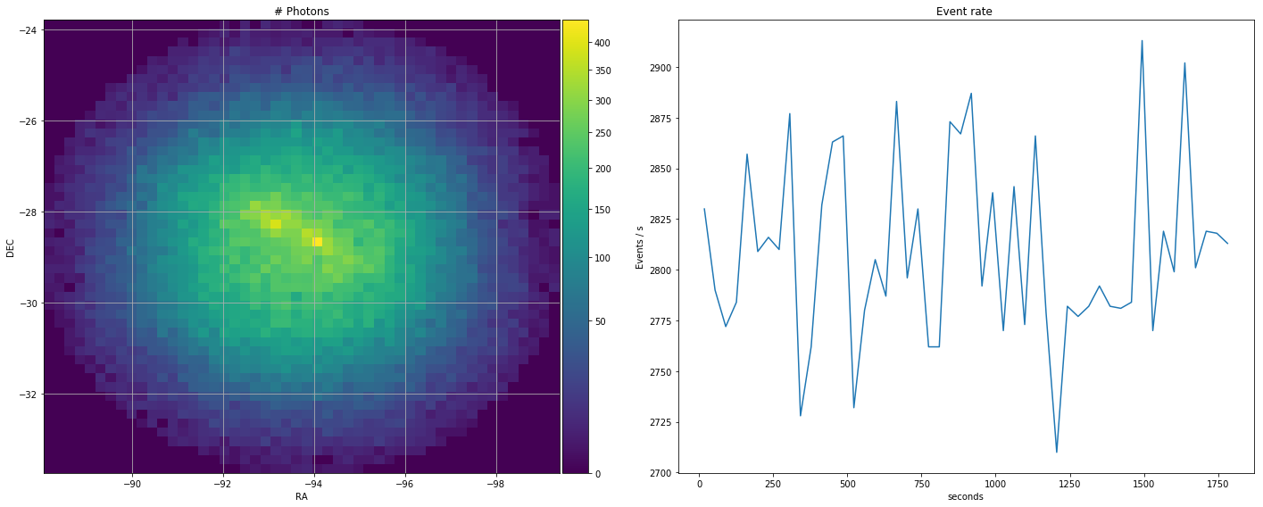
events = obs.events
events.peek()
events.table[:5][['EVENT_ID', 'TIME', 'ENERGY', 'RA', 'DEC']]
Out[9]:
| EVENT_ID | TIME | ENERGY | RA | DEC |
|---|---|---|---|---|
| s | TeV | deg | deg | |
| uint32 | float64 | float32 | float32 | float32 |
| 1 | 665735041.7 | 0.0384564 | -92.6261 | -28.4639 |
| 2 | 665735042.72 | 0.0407098 | -92.307 | -27.1749 |
| 3 | 665735042.878 | 0.0429804 | -93.4977 | -28.7857 |
| 4 | 665735045.849 | 0.0411471 | -92.9102 | -27.9038 |
| 5 | 665735057.423 | 0.0347661 | -94.1769 | -29.147 |

Effective area
Explore EffectiveAreaTable2d and EffectiveAreaTable
In [10]:
aeff = obs.aeff
aeff.peek()
print(aeff)
<gammapy.irf.effective_area.EffectiveAreaTable2D object at 0x111bc5160>

In [11]:
# Slice out effective area at a given offset
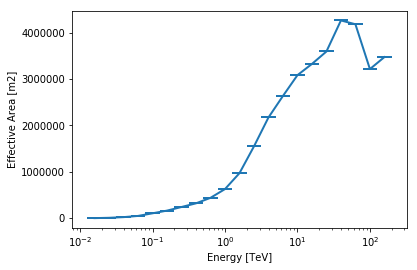
effarea = aeff.to_effective_area_table(offset=0.5 * u.deg)
effarea.plot()
Out[11]:
<matplotlib.axes._subplots.AxesSubplot at 0x110418048>

Energy dispersion
Explore EnergyDispersion2d and EnergyDispersion
In [12]:
edisp = obs.edisp
edisp.peek()
print(edisp)
/opt/local/Library/Frameworks/Python.framework/Versions/3.5/lib/python3.5/site-packages/matplotlib/colors.py:1152: UserWarning: Power-law scaling on negative values is ill-defined, clamping to 0.
  warnings.warn("Power-law scaling on negative values is "
/Users/deil/Library/Python/3.5/lib/python/site-packages/astropy/units/quantity.py:951: RuntimeWarning: invalid value encountered in true_divide
  return super(Quantity, self).__truediv__(other)
EnergyDispersion2D
NDDataArray summary info
e_true         : size =    60, min =  0.011 TeV, max = 8912.510 TeV
migra          : size =   300, min =  0.005, max =  2.995
offset         : size =     6, min =  0.500 deg, max =  5.500 deg
Data           : size = 108000, min =  0.000, max = 913.000
/opt/local/Library/Frameworks/Python.framework/Versions/3.5/lib/python3.5/site-packages/matplotlib/colors.py:1113: RuntimeWarning: invalid value encountered in power
  np.power(resdat, gamma, resdat)

In [13]:
# Calculate energy dispersion matrix at a given offset
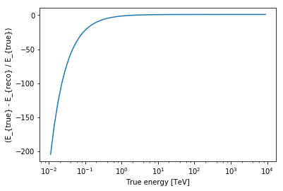
response_matrix = edisp.to_energy_dispersion(offset=0.5 * u.deg)
response_matrix.plot_bias()
/Users/deil/Library/Python/3.5/lib/python/site-packages/astropy/units/quantity.py:951: RuntimeWarning: invalid value encountered in true_divide
  return super(Quantity, self).__truediv__(other)
Out[13]:
<matplotlib.axes._subplots.AxesSubplot at 0x11040bb38>

PSF
TODO: examples for point spread function (PSF)
In [14]:
psf = obs.psf
psf.peek()
print(psf)
No safe energy thresholds found. Setting to default
/Users/deil/Library/Python/3.5/lib/python/site-packages/gammapy/image/models/gauss.py:254: RuntimeWarning: invalid value encountered in true_divide
  self.norms /= self.integral
<gammapy.irf.psf_analytical.EnergyDependentMultiGaussPSF object at 0x10de9bfd0>
/opt/local/Library/Frameworks/Python.framework/Versions/3.5/lib/python3.5/site-packages/matplotlib/colors.py:494: RuntimeWarning: invalid value encountered in less
  cbook._putmask(xa, xa < 0.0, -1)

Background model
TODO: example how to load and plot
gammapy.background.FOVBackgroundModel
In [17]:
# TODO: doesn't work yet
# bkg = obs.bkg
# bkg.peek()
# print(bkg)
What next?
In this tutorial we have learned how to access and check IACT DL3 data.
Usually for a science analysis, if others have checked the data and IRF quality for you and you trust it’s good, you don’t need to do that. Instead, you’ll just run an analysis and look at higher-level results, like images or spectra.
Next you could do:
- image analysis
- spectral analysis
- cube analysis
- time analysis
- source detection