This is a fixed-text formatted version of a Jupyter notebook.
You can contribute with your own notebooks in this GitHub repository.
Source files: detect_ts.ipynb | detect_ts.py
Source detection with Gammapy
Introduction
This notebook show how to do source detection with Gammapy. using one of the methods available in gammapy.detect.
We will do this:
- produce 2-dimensional test-statistics (TS) images using Fermi-LAT 2FHL high-energy Galactic plane survey dataset
- run a peak finder to make a source catalog
- do some simple measurements on each source
- compare to the 2FHL catalog
Note that what we do here is a quick-look analysis. Producing a real source catalog for Fermi-LAT, HGPS or CTA is a more elaborate procedure.
We will work with the following functions and classes:
- photutils and specifically the photutils.detection.find_peaks function.
- gammapy.image.SkyImage
- gammapy.image.SkyImageList
- gammapy.detect.TSImageEstimator
Setup
As always, let’s get started with some setup …
In [1]:
%matplotlib inline
import matplotlib.pyplot as plt
In [2]:
from astropy import units as u
from astropy.convolution import Gaussian2DKernel
from astropy.coordinates import SkyCoord

from photutils.detection import find_peaks

from gammapy.image import SkyImageList
from gammapy.detect import TSImageEstimator
from gammapy.catalog import source_catalogs
Compute TS image
In [3]:
# Load data from files
images = SkyImageList.read('../datasets/fermi_survey/all.fits.gz')
images['COUNTS'].name = 'counts'
images['BACKGROUND'].name = 'background'
images['EXPOSURE'].name = 'exposure'
In [4]:
# Compute a source kernel (source template) in oversample mode,
# PSF is not taken into account
kernel = Gaussian2DKernel(2.5, mode='oversample')

# Compute a TS map. 'On' is the raw counts map, 'Background' is the background model,
# 'ExpGammaMap' denotes to the exposure map.
estimator = TSImageEstimator()
result = estimator.run(images, kernel)

print('TS map computation took {0:.2f} s'.format(result.meta['runtime']))
TS map computation took 8.97 s
Plot images
In [5]:
# Plot sqrt(TS) map
fig_ts = plt.figure(figsize=(18, 4))
ax_ts = fig_ts.add_axes([0.1, 0.1, 0.9, 0.9], projection=images['counts'].wcs)
ax_ts.imshow(result['sqrt_ts'], cmap='afmhot', origin='lower', vmin=0, vmax=10)
ax_ts.coords['glon'].set_axislabel('Galactic Longitude')
ax_ts.coords['glat'].set_axislabel('Galactic Latitude')

In [6]:
# Plot flux map (in units of m^-2 s^-1 TeV^-1)
fig_flux = plt.figure(figsize=(18, 4))
ax_flux = fig_flux.add_axes([0.1, 0.1, 0.9, 0.9], projection=images['counts'].wcs)
ax_flux.imshow(result['flux'], cmap='afmhot', origin='lower', vmin=0, vmax=1E-9)
ax_flux.coords['glon'].set_axislabel('Galactic Longitude')
ax_flux.coords['glat'].set_axislabel('Galactic Latitude')

In [7]:
# Plot number of iterations of the fit per pixel
fig_iter = plt.figure(figsize=(18, 4))
ax_iter = fig_iter.add_axes([0.1, 0.1, 0.9, 0.9], projection=images['counts'].wcs)
ax_iter.imshow(result['niter'], cmap='afmhot', origin='lower', vmin=0, vmax=20)
ax_iter.coords['glon'].set_axislabel('Galactic Longitude')
ax_iter.coords['glat'].set_axislabel('Galactic Latitude')

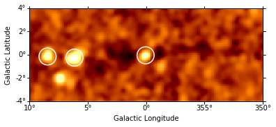
Source catalog
Let’s run a peak finder on the sqrt_ts image to get a list of
sources (positions and peak sqrt_ts values).
In [8]:
sources = find_peaks(
    data=result['sqrt_ts'].data,
    threshold=10,
    wcs=result['sqrt_ts'].wcs,
)
sources
/opt/local/Library/Frameworks/Python.framework/Versions/3.6/lib/python3.6/site-packages/photutils/detection/core.py:241: RuntimeWarning: invalid value encountered in greater
  peak_goodmask = np.logical_and(peak_goodmask, (data > threshold))
Out[8]:
| x_peak | y_peak | icrs_ra_peak | icrs_dec_peak | peak_value |
|---|---|---|---|---|
| deg | deg | |||
| int64 | int64 | float64 | float64 | float64 |
| 1965 | 22 | 128.763048393 | -45.2123926707 | 86.9619775881 |
| 1169 | 23 | 257.543796578 | -44.4818050084 | 30.5466752124 |
| 1338 | 33 | 238.171431899 | -56.1850306688 | 11.0775144301 |
| 1943 | 35 | 132.164175646 | -46.1492131281 | 10.5063691882 |
| 1934 | 36 | 133.10541837 | -46.7809911803 | 10.5550153527 |
| 1397 | 38 | 228.619705559 | -59.1959453409 | 10.9478617214 |
| 1724 | 44 | 161.339190999 | -59.7273459329 | 15.2158412054 |
| 509 | 46 | 290.82410573 | 14.1806184739 | 15.3210531504 |
| 1749 | 46 | 157.300019886 | -58.323296616 | 10.6092905189 |
| 1758 | 47 | 155.953257132 | -57.7647878196 | 10.2275638537 |
| 939 | 48 | 270.135282158 | -23.7665329915 | 11.3860517586 |
| 916 | 49 | 271.270506536 | -21.7161746387 | 10.0442662879 |
| 1000 | 50 | 266.483508145 | -28.9195295409 | 10.0077744483 |
| 1236 | 52 | 248.150530438 | -47.7993631076 | 12.9367404988 |
| 218 | 73 | 305.219107925 | 40.557774537 | 15.5937483251 |
| 1279 | 77 | 240.882704747 | -49.0114152369 | 12.6880775192 |
In [9]:
# Plot sources on top of significance sky image
result['sqrt_ts'].cutout(
    position=SkyCoord(0, 0, unit='deg', frame='galactic'),
    size=(8*u.deg, 20*u.deg)
).plot()

plt.gca().scatter(
    sources['icrs_ra_peak'], sources['icrs_dec_peak'],
    transform=plt.gca().get_transform('icrs'),
    color='none', edgecolor='white', marker='o', s=600, lw=1.5,
)
Out[9]:
<matplotlib.collections.PathCollection at 0x11556d320>

Measurements
- TODO: show cutout for a few sources and some aperture photometry measurements (e.g. energy distribution, significance, flux)
In [10]:
# TODO
Compare to 2FHL
TODO
In [11]:
fermi_2fhl = source_catalogs['2fhl']
fermi_2fhl.table[:5][['Source_Name', 'GLON', 'GLAT']]
Out[11]:
| Source_Name | GLON | GLAT |
|---|---|---|
| deg | deg | |
| str18 | float32 | float32 |
| 2FHL J0008.1+4709 | 115.339 | -15.0688 |
| 2FHL J0009.3+5031 | 116.124 | -11.7932 |
| 2FHL J0018.5+2947 | 114.463 | -32.5424 |
| 2FHL J0022.0+0006 | 107.172 | -61.8618 |
| 2FHL J0033.6-1921 | 94.28 | -81.2224 |
What next?
In this notebook, we have seen how to work with images and compute TS images from counts data, if a background estimate is already available.
Here’s some suggestions what to do next:
- TODO: point to background estimation examples
- TODO: point to other docs …