This is a fixed-text formatted version of a Jupyter notebook.
You can contribute with your own notebooks in this GitHub repository.
Source files: spectrum_simulation.ipynb | spectrum_simulation.py
Spectrum simulation with Gammapy
Introduction
This notebook explains how to use the functions and classes in gammapy.spectrum in order to simulate and fit spectra.
First, we will simulate and fit a pure power law without any background. Than we will add a power law shaped background component. Finally, we will see how to simulate and fit a user defined model. For all scenarios a toy detector will be simulated. For an example using real CTA IRFs, checkout this notebook.
The following clases will be used:
- gammapy.irf.EffectiveAreaTable
- gammapy.irf.EnergyDispersion
- gammapy.spectrum.SpectrumObservation
- gammapy.spectrum.SpectrumSimulation
- gammapy.spectrum.SpectrumFit
- gammapy.spectrum.models.PowerLaw
- gammapy.spectrum.models.SpectralModel
Feedback welcome!
Setup
Same procedure as in every script …
In [1]:
%matplotlib inline
import matplotlib.pyplot as plt
In [2]:
import numpy as np
import astropy.units as u
from gammapy.irf import EnergyDispersion, EffectiveAreaTable
from gammapy.spectrum import SpectrumSimulation, SpectrumFit
from gammapy.spectrum.models import PowerLaw, SpectralModel
from gammapy.utils.modeling import Parameter, ParameterList
Create detector
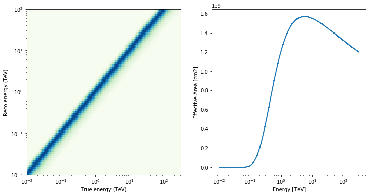
For the sake of self consistency of this tutorial, we will simulate a simple detector. For a real application you would want to replace this part of the code with loading the IRFs or your detector (TODO: Link to IRFs tutorial)
In [3]:
e_true = np.logspace(-2, 2.5, 109) * u.TeV
e_reco = np.logspace(-2,2, 79) * u.TeV

edisp = EnergyDispersion.from_gauss(e_true=e_true, e_reco=e_reco, sigma=0.2, bias=0)
aeff = EffectiveAreaTable.from_parametrization(energy=e_true)

fig, axes = plt.subplots(1, 2, figsize=(12, 6))
edisp.plot_matrix(ax=axes[0])
aeff.plot(ax=axes[1])
Out[3]:
<matplotlib.axes._subplots.AxesSubplot at 0x1095022e8>

Power law
In this section we will simulate one observation using a power law model.
In [4]:
index = 2.3 * u.Unit('')
amplitude = 1e-11 * u.Unit('cm-2 s-1 TeV-1')
reference = 1 * u.TeV

pwl = PowerLaw(index=index, amplitude=amplitude, reference=reference)
print(pwl)

livetime = 2 * u.h
PowerLaw

Parameters:

           name     value   error       unit      min max frozen
        --------- --------- ----- --------------- --- --- ------
            index 2.300e+00   nan                 nan nan  False
        amplitude 1.000e-11   nan 1 / (cm2 s TeV) nan nan  False
        reference 1.000e+00   nan             TeV nan nan   True
In [5]:
sim = SpectrumSimulation(aeff=aeff,
                         edisp=edisp,
                         source_model=pwl,
                         livetime=livetime)
sim.simulate_obs(seed=2309, obs_id=1)
print(sim.obs)
*** Observation summary report ***
Observation Id: 1
Livetime: 2.000 h
On events: 339
Off events: 0
Alpha: 1.000
Bkg events in On region: 0.00
Excess: 339.00
Excess / Background: inf
Gamma rate: 0.04 1 / min
Bkg rate: 0.00 1 / min
Sigma: nan
energy range: 0.01 TeV - 100.00 TeV
/Users/deil/code/gammapy/gammapy/data/obs_stats.py:209: RuntimeWarning: divide by zero encountered in true_divide
  self.background))
/Users/deil/code/gammapy/gammapy/stats/poisson.py:385: RuntimeWarning: divide by zero encountered in log
  m = n_off * log(n_off * temp)
/Users/deil/code/gammapy/gammapy/stats/poisson.py:385: RuntimeWarning: invalid value encountered in multiply
  m = n_off * log(n_off * temp)
In [6]:
fit = SpectrumFit(obs_list=sim.obs, model=pwl.copy(), stat='cash')
fit.fit_range = [1, 10] * u.TeV
fit.fit()
fit.est_errors()
print(fit.result[0])
Fit result info
---------------
Model: PowerLaw

Parameters:

           name     value     error         unit      min max frozen
        --------- --------- --------- --------------- --- --- ------
            index 2.259e+00 2.192e-01                 nan nan  False
        amplitude 9.255e-12 1.755e-12 1 / (cm2 s TeV) nan nan  False
        reference 1.000e+00 0.000e+00             TeV nan nan   True

Covariance:

        name/name  index   amplitude
        --------- -------- ---------
            index   0.0481  2.99e-13
        amplitude 2.99e-13  3.08e-24

Statistic: -74.059 (cash)
Fit Range: [ 1.          9.42668455] TeV
Include background
In this section we will include a background component. Furthermore, we will also simulate more than one observation and fit each one individuallt in order to get average fit results.
In [7]:
bkg_index = 2.5 * u.Unit('')
bkg_amplitude = 1e-11 * u.Unit('cm-2 s-1 TeV-1')
reference = 1 * u.TeV

bkg_model = PowerLaw(index=bkg_index, amplitude=bkg_amplitude, reference=reference)
alpha = 0.2
In [8]:
n_obs = 10
seeds = np.arange(n_obs)

sim = SpectrumSimulation(aeff=aeff,
                         edisp=edisp,
                         source_model=pwl,
                         livetime=livetime,
                         background_model=bkg_model,
                         alpha=alpha)

sim.run(seeds)
print(sim.result)
print(sim.result[0])
SpectrumObservationList
Number of observations: 10
*** Observation summary report ***
Observation Id: 0
Livetime: 2.000 h
On events: 733
Off events: 1915
Alpha: 0.200
Bkg events in On region: 383.00
Excess: 350.00
Excess / Background: 0.91
Gamma rate: 0.04 1 / min
Bkg rate: 0.04 1 / min
Sigma: 14.17
energy range: 0.01 TeV - 100.00 TeV
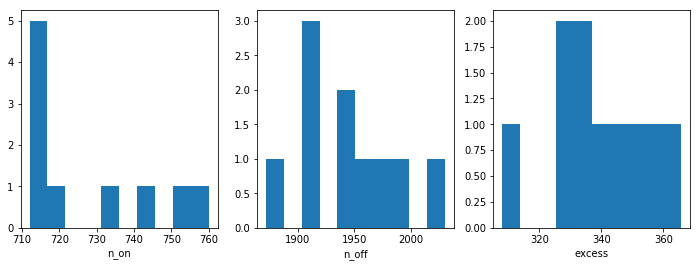
Before moving on to the fit let’s have a look at the simulated observations
In [9]:
n_on = [obs.total_stats.n_on for obs in sim.result]
n_off = [obs.total_stats.n_off for obs in sim.result]
excess = [obs.total_stats.excess for obs in sim.result]

fix, axes = plt.subplots(1,3, figsize=(12, 4))
axes[0].hist(n_on)
axes[0].set_xlabel('n_on')
axes[1].hist(n_off)
axes[1].set_xlabel('n_off')
axes[2].hist(excess)
axes[2].set_xlabel('excess')
Out[9]:
<matplotlib.text.Text at 0x10a012c50>

In [10]:
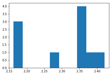
best_fit_index = []

pwl.parameters['index'].parmax = 10
for obs in sim.result:
    fit = SpectrumFit(obs, pwl.copy(), stat='wstat')
    fit.model.parameters['index'].value = 2
    fit.fit()
    best_fit_index.append(fit.result[0].model.parameters['index'].value)
/Users/deil/code/gammapy/gammapy/stats/fit_statistics.py:166: RuntimeWarning: divide by zero encountered in log
  term3_ = - n_off * np.log(mu_bkg)
/Users/deil/code/gammapy/gammapy/stats/fit_statistics.py:203: RuntimeWarning: divide by zero encountered in log
  term1 = - n_on * (1 - np.log(n_on))
/Users/deil/code/gammapy/gammapy/stats/fit_statistics.py:204: RuntimeWarning: divide by zero encountered in log
  term2 = - n_off * (1 - np.log(n_off))
/Users/deil/code/gammapy/gammapy/stats/fit_statistics.py:161: RuntimeWarning: divide by zero encountered in log
  term2_ = - n_on * np.log(mu_sig + alpha * mu_bkg)
In [11]:
plt.hist(best_fit_index)
print('best_fit_index:', best_fit_index)
best_fit_index: [2.4210876310429703, 2.348343811183434, 2.3452606874153705, 2.2849302714618704, 2.1708828724555853, 2.1624319913222068, 2.3647918746839056, 2.3849072419290813, 2.3691150798628171, 2.1822751318255573]

Exercises
- Fit a pure power law and the user define model to the observation you just simulated. You can start with the user defined model described in the spectrum_models.ipynb notebook.
- Vary the observation lifetime and see when you can distinguish the two models (Hint: You get the final likelihood of a fit from fit.result[0].statval).
What’s next
In this tutorial we learnd how to simulate and fit data using a toy detector. Go to gammapy.spectrum to see what else you can do with gammapy.