This is a fixed-text formatted version of a Jupyter notebook.
You can contribute with your own notebooks in this GitHub repository.
Source files: sed_fitting_gammacat_fermi.ipynb | sed_fitting_gammacat_fermi.py
Flux point fitting in Gammapy
Introduction
In this tutorial we’re going to learn how to fit spectral models to combined Fermi-LAT and IACT flux points.
The central class we’re going to use for this example analysis is:
In addition we will work with the following data classes:
- gammapy.spectrum.FluxPoints
- gammapy.catalog.SourceCatalogGammaCat
- gammapy.catalog.SourceCatalog3FHL
- gammapy.catalog.SourceCatalog3FGL
And the following spectral model classes:
Setup
Let us start with the usual IPython notebook and Python imports:
In [1]:
%matplotlib inline
import numpy as np
import matplotlib.pyplot as plt
In [2]:
from astropy import units as u
from astropy.table import vstack
from gammapy.spectrum.models import PowerLaw, ExponentialCutoffPowerLaw, LogParabola
from gammapy.spectrum import FluxPointFitter, FluxPoints
from gammapy.catalog import SourceCatalog3FGL, SourceCatalogGammaCat, SourceCatalog3FHL
Load spectral points
For this analysis we choose to work with the source ‘HESS J1507-622’ and the associated Fermi-LAT sources ‘3FGL J1506.6-6219’ and ‘3FHL J1507.9-6228e’. We load the source catalogs, and then access source of interest by name:
In [3]:
fermi_3fgl = SourceCatalog3FGL()
fermi_3fhl = SourceCatalog3FHL()
gammacat = SourceCatalogGammaCat()
In [4]:
source_gammacat =  gammacat['HESS J1507-622']
source_fermi_3fgl = fermi_3fgl['3FGL J1506.6-6219']
source_fermi_3fhl = fermi_3fhl['3FHL J1507.9-6228e']
The corresponding flux points data can be accessed with .flux_points
attribute:
In [5]:
flux_points_gammacat = source_gammacat.flux_points
flux_points_gammacat.table
Out[5]:
| e_ref | dnde | dnde_errn | dnde_errp |
|---|---|---|---|
| TeV | 1 / (cm2 s TeV) | 1 / (cm2 s TeV) | 1 / (cm2 s TeV) |
| float32 | float32 | float32 | float32 |
| 0.8609 | 2.29119e-12 | 8.70543e-13 | 8.95502e-13 |
| 1.56151 | 6.98172e-13 | 2.20354e-13 | 2.30407e-13 |
| 2.76375 | 1.69062e-13 | 6.7587e-14 | 7.18838e-14 |
| 4.8916 | 7.72925e-14 | 2.40132e-14 | 2.60749e-14 |
| 9.98858 | 1.03253e-14 | 5.06315e-15 | 5.64195e-15 |
| 27.0403 | 7.44987e-16 | 5.72089e-16 | 7.25999e-16 |
In the Fermi-LAT catalogs, integral flux points are given. Currently the flux point fitter only works with differential flux points, so we apply the conversion here.
In [6]:
flux_points_3fgl = source_fermi_3fgl.flux_points.to_sed_type(
    sed_type='dnde',
    model=source_fermi_3fgl.spectral_model,
)
flux_points_3fhl = source_fermi_3fhl.flux_points.to_sed_type(
    sed_type='dnde',
    model=source_fermi_3fhl.spectral_model,
)
Finally we stack the flux points into a single FluxPoints object and
drop the upper limit values, because currently we can’t handle them in
the fit:
In [7]:
# stack flux point tables
flux_points = FluxPoints.stack([
    flux_points_gammacat,
    flux_points_3fhl,
    flux_points_3fgl
])

# drop the flux upper limit values
flux_points = flux_points.drop_ul()
Fitter Setup
We initialze the fitter object with the 'chi2assym' statistic,
because we have assymmetric errors on the flux points. As optimizer we
choose the 'simplex' algorithm and to estimate the errors we use
'covar' method:
In [8]:
fitter = FluxPointFitter(
    stat='chi2assym',
    optimizer='simplex',
    error_estimator='covar',
)
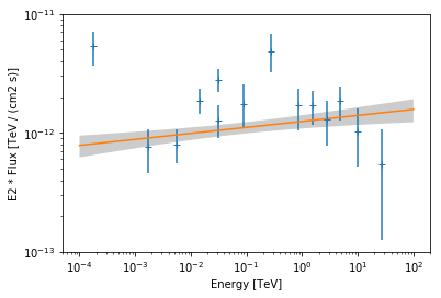
Power Law Fit
First we start with fitting a simple power law.
In [9]:
pwl = PowerLaw(
    index=2. * u.Unit(''),
    amplitude=1e-12 * u.Unit('cm-2 s-1 TeV-1'),
    reference=1. * u.TeV
)
After creating the model we run the fit by passing the 'flux_points'
and 'pwl' objects:
In [10]:
result_pwl = fitter.run(flux_points, pwl)
And print the result:
In [11]:
print(result_pwl['best-fit-model'])
PowerLaw

Parameters:

           name     value     error         unit      min max frozen
        --------- --------- --------- --------------- --- --- ------
            index 1.950e+00 2.656e-02                 nan nan  False
        amplitude 1.248e-12 1.599e-13 1 / (cm2 s TeV) nan nan  False
        reference 1.000e+00 0.000e+00             TeV nan nan   True

Covariance:

        name/name   index   amplitude
        --------- --------- ---------
            index  0.000706 -2.25e-15
        amplitude -2.25e-15  2.56e-26
As a quick check we print the value of the fit statistics per degrees of freedom as well:
In [12]:
print(result_pwl['statval/dof'])
2.5038842921602655
Finally we plot the data points and the best fit model:
In [13]:
ax = flux_points.plot(energy_power=2)
result_pwl['best-fit-model'].plot(energy_range=[1e-4, 1e2] * u.TeV, ax=ax, energy_power=2)
result_pwl['best-fit-model'].plot_error(energy_range=[1e-4, 1e2] * u.TeV, ax=ax, energy_power=2)
ax.set_ylim(1e-13, 1e-11)
Out[13]:
(1e-13, 1e-11)
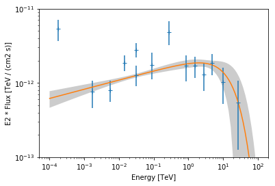
Exponential Cut-Off Powerlaw Fit
Next we fit an exponential cut-off power law to the data.
In [14]:
ecpl = ExponentialCutoffPowerLaw(
    index=2. * u.Unit(''),
    amplitude=1e-12 * u.Unit('cm-2 s-1 TeV-1'),
    reference=1. * u.TeV,
    lambda_=0. / u.TeV
)
We run the fitter again by passing the flux points and the ecpl
model instance:
In [15]:
result_ecpl = fitter.run(flux_points, ecpl)
print(result_ecpl['best-fit-model'])
ExponentialCutoffPowerLaw

Parameters:

           name     value     error         unit      min max frozen
        --------- --------- --------- --------------- --- --- ------
            index 1.876e+00 4.388e-02                 nan nan  False
        amplitude 1.932e-12 3.873e-13 1 / (cm2 s TeV) nan nan  False
        reference 1.000e+00 0.000e+00             TeV nan nan   True
          lambda_ 6.147e-02 5.795e-02         1 / TeV nan nan  False

Covariance:

        name/name   index   amplitude lambda_
        --------- --------- --------- --------
            index   0.00193 -1.35e-14 -0.00178
        amplitude -1.35e-14   1.5e-25 1.73e-14
          lambda_  -0.00178  1.73e-14  0.00336
In [16]:
print(result_ecpl['statval/dof'])
2.001353939388082
We plot the data and best fit model:
In [17]:
ax = flux_points.plot(energy_power=2)
result_ecpl['best-fit-model'].plot(energy_range=[1e-4, 1e2] * u.TeV, ax=ax, energy_power=2)
result_ecpl['best-fit-model'].plot_error(energy_range=[1e-4, 1e2] * u.TeV, ax=ax, energy_power=2)
ax.set_ylim(1e-13, 1e-11)
Out[17]:
(1e-13, 1e-11)
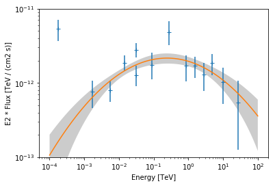
Log-Parabola Fit
Finally we try to fit a log-parabola model:
In [18]:
log_parabola = LogParabola(
    alpha=2. * u.Unit(''),
    amplitude=1e-12 * u.Unit('cm-2 s-1 TeV-1'),
    reference=1. * u.TeV,
    beta=0. * u.Unit('')
)
In [19]:
result_log_parabola = fitter.run(flux_points, log_parabola)
print(result_log_parabola['best-fit-model'])
LogParabola

Parameters:

           name     value     error         unit      min max frozen
        --------- --------- --------- --------------- --- --- ------
        amplitude 1.954e-12 2.797e-13 1 / (cm2 s TeV) nan nan  False
        reference 1.000e+00 0.000e+00             TeV nan nan   True
            alpha 2.140e+00 7.377e-02                 nan nan  False
             beta 4.947e-02 1.757e-02                 nan nan  False

Covariance:

        name/name amplitude  alpha     beta
        --------- --------- -------- --------
        amplitude  7.82e-26 1.79e-15 2.19e-15
            alpha  1.79e-15  0.00544  0.00112
             beta  2.19e-15  0.00112 0.000309
In [20]:
print(result_log_parabola['statval/dof'])
1.5798902196277185
In [21]:
ax = flux_points.plot(energy_power=2)
result_log_parabola['best-fit-model'].plot(energy_range=[1e-4, 1e2] * u.TeV, ax=ax, energy_power=2)
result_log_parabola['best-fit-model'].plot_error(energy_range=[1e-4, 1e2] * u.TeV, ax=ax, energy_power=2)
ax.set_ylim(1e-13, 1e-11)
Out[21]:
(1e-13, 1e-11)
Exercises
- Fit a
PowerLaw2andExponentialCutoffPowerLaw3FGLto the same data. - Fit a
ExponentialCutoffPowerLawmodel to Vela X (‘HESS J0835-455’) only and check if the best fit values correspond to the values given in the Gammacat catalog
What next?
This was an introduction to SED fitting in Gammapy.
- If you would like to learn how to perform a full Poisson maximum likelihood spectral fit, please check out the spectrum pipe tutorial.
- If you are interested in simulation of spectral data in the context of CTA, please check out the spectrum simulation cta notebook.
- To learn more about other parts of Gammapy (e.g. Fermi-LAT and TeV data analysis), check out the other tutorial notebooks.
- To see what’s available in Gammapy, browse the Gammapy docs or use the full-text search.
- If you have any questions, ask on the mailing list .