This is a fixed-text formatted version of a Jupyter notebook.
You can contribute with your own notebooks in this GitHub repository.
Source files: spectrum_pipe.ipynb | spectrum_pipe.py
Spectrum analysis with Gammapy (run pipeline)
In this tutorial we will learn how to perform a 1d spectral analysis.
We will use a “pipeline” or “workflow” class to run a standard analysis. If you’re interested in implementation detail of the analysis in order to create a custom analysis class, you should read (spectrum_analysis.ipynb) that executes the analysis using lower-level classes and methods in Gammapy.
In this tutorial we will use the folling Gammapy classes:
- gammapy.data.DataStore to load the data to
- gammapy.scripts.SpectrumAnalysisIACT to run the analysis
We use 4 Crab observations from H.E.S.S. for testing.
Setup
As usual, we’ll start with some setup for the notebook, and import the functionality we need.
In [1]:
%matplotlib inline
import numpy as np
import matplotlib.pyplot as plt

from gammapy.data import DataStore
from gammapy.scripts import SpectrumAnalysisIACT

# Convenience classes to define analsys inputs
# At some point we'll add a convenience layer to run the analysis starting from a plain text config file.
from gammapy.utils.energy import EnergyBounds
from gammapy.image import SkyImage
from gammapy.spectrum import models
from regions import CircleSkyRegion
from astropy.coordinates import SkyCoord
import astropy.units as u
Select data
First, we select and load some H.E.S.S. data (simulated events for now). In real life you would do something fancy here, or just use the list of observations someone send you (and hope they have done something fancy before). We’ll just use the standard gammapy 4 crab runs.
In [2]:
# TODO: Replace with public data release
store_dir = '$GAMMAPY_EXTRA/datasets/hess-crab4-hd-hap-prod2'
data_store = DataStore.from_dir(store_dir)
obs_id = data_store.obs_table['OBS_ID'].data
print("Use observations {}".format(obs_id))

obs_list = data_store.obs_list(obs_id)
Use observations [23523 23526 23559 23592]
Configure the analysis
Now we’ll define the input for the spectrum analysis. It will be done the python way, i.e. by creating a config dict containing python objects. We plan to add also the convenience to configure the analysis using a plain text config file.
In [3]:
crab_pos = SkyCoord.from_name('crab')
on_region = CircleSkyRegion(crab_pos, 0.15 * u.deg)

model = models.LogParabola(
    alpha = 2.3,
    beta = 0,
    amplitude = 1e-11 * u.Unit('cm-2 s-1 TeV-1'),
    reference = 1 * u.TeV,
)

flux_point_binning = EnergyBounds.equal_log_spacing(0.7, 30, 5, u.TeV)

exclusion_mask = SkyImage.read('$GAMMAPY_EXTRA/datasets/exclusion_masks/tevcat_exclusion.fits')
In [4]:
config = dict(
    outdir = None,
    background = dict(
        on_region=on_region,
        exclusion_mask=exclusion_mask,
        min_distance = 0.1 * u.rad,
    ),
    extraction = dict(containment_correction=False),
    fit = dict(
        model=model,
        stat='wstat',
        forward_folded=True,
        fit_range = flux_point_binning[[0, -1]]
    ),
    fp_binning=flux_point_binning
)
Run the analysis
TODO: Clean up the log (partly done, get rid of remaining useless warnings)
In [5]:
ana = SpectrumAnalysisIACT(
    observations=obs_list,
    config=config,
)
ana.run()
INFO:gammapy.scripts.spectrum_pipe:Running SpectrumAnalysisIACT
INFO:gammapy.background.reflected:Running ReflectedRegionsBackgroundEstimator
Region: CircleSkyRegion
center: <SkyCoord (ICRS): (ra, dec) in deg
    ( 83.633212,  22.01446)>
radius: 0.15 deg
ObservationList
Number of observations: 4
Info for OBS_ID = 23523
- Start time: 53343.92
- Pointing pos: RA 83.63 deg / Dec 21.51 deg
- Observation duration: 1687.0 s
- Dead-time fraction: 6.240 %
Info for OBS_ID = 23526
- Start time: 53343.95
- Pointing pos: RA 83.63 deg / Dec 22.51 deg
- Observation duration: 1683.0 s
- Dead-time fraction: 6.555 %
Info for OBS_ID = 23559
- Start time: 53345.96
- Pointing pos: RA 85.25 deg / Dec 22.01 deg
- Observation duration: 1686.0 s
- Dead-time fraction: 6.398 %
Info for OBS_ID = 23592
- Start time: 53347.91
- Pointing pos: RA 82.01 deg / Dec 22.01 deg
- Observation duration: 1686.0 s
- Dead-time fraction: 6.212 %

<gammapy.background.reflected.ReflectedRegionsFinder object at 0x11246b5c0>
INFO:gammapy.background.reflected:Processing observation Info for OBS_ID = 23523
- Start time: 53343.92
- Pointing pos: RA 83.63 deg / Dec 21.51 deg
- Observation duration: 1687.0 s
- Dead-time fraction: 6.240 %

INFO:gammapy.background.reflected:Found 7 reflected regions
INFO:gammapy.background.reflected:Processing observation Info for OBS_ID = 23526
- Start time: 53343.95
- Pointing pos: RA 83.63 deg / Dec 22.51 deg
- Observation duration: 1683.0 s
- Dead-time fraction: 6.555 %

INFO:gammapy.background.reflected:Found 7 reflected regions
INFO:gammapy.background.reflected:Processing observation Info for OBS_ID = 23559
- Start time: 53345.96
- Pointing pos: RA 85.25 deg / Dec 22.01 deg
- Observation duration: 1686.0 s
- Dead-time fraction: 6.398 %

INFO:gammapy.background.reflected:Found 19 reflected regions
INFO:gammapy.background.reflected:Processing observation Info for OBS_ID = 23592
- Start time: 53347.91
- Pointing pos: RA 82.01 deg / Dec 22.01 deg
- Observation duration: 1686.0 s
- Dead-time fraction: 6.212 %

INFO:gammapy.background.reflected:Found 17 reflected regions
INFO:gammapy.spectrum.extract:Running <gammapy.spectrum.extract.SpectrumExtraction object at 0x1119d0080>
INFO:gammapy.spectrum.extract:Process observation
 Info for OBS_ID = 23523
- Start time: 53343.92
- Pointing pos: RA 83.63 deg / Dec 21.51 deg
- Observation duration: 1687.0 s
- Dead-time fraction: 6.240 %

INFO:gammapy.spectrum.extract:Update observation meta info
INFO:gammapy.spectrum.extract:Offset : 0.5000156610786867 deg

INFO:gammapy.spectrum.extract:Fill events
INFO:gammapy.spectrum.extract:Extract IRFs
/Users/deil/Library/Python/3.6/lib/python/site-packages/astropy/units/quantity.py:634: RuntimeWarning: invalid value encountered in true_divide
  result = super().__array_ufunc__(function, method, *arrays, **kwargs)
INFO:gammapy.spectrum.extract:Process observation
 Info for OBS_ID = 23526
- Start time: 53343.95
- Pointing pos: RA 83.63 deg / Dec 22.51 deg
- Observation duration: 1683.0 s
- Dead-time fraction: 6.555 %

INFO:gammapy.spectrum.extract:Update observation meta info
INFO:gammapy.spectrum.extract:Offset : 0.4999843633857045 deg

INFO:gammapy.spectrum.extract:Fill events
INFO:gammapy.spectrum.extract:Extract IRFs
INFO:gammapy.spectrum.extract:Process observation
 Info for OBS_ID = 23559
- Start time: 53345.96
- Pointing pos: RA 85.25 deg / Dec 22.01 deg
- Observation duration: 1686.0 s
- Dead-time fraction: 6.398 %

INFO:gammapy.spectrum.extract:Update observation meta info
INFO:gammapy.spectrum.extract:Offset : 1.501990838622691 deg

INFO:gammapy.spectrum.extract:Fill events
INFO:gammapy.spectrum.extract:Extract IRFs
INFO:gammapy.spectrum.extract:Process observation
 Info for OBS_ID = 23592
- Start time: 53347.91
- Pointing pos: RA 82.01 deg / Dec 22.01 deg
- Observation duration: 1686.0 s
- Dead-time fraction: 6.212 %

INFO:gammapy.spectrum.extract:Update observation meta info
INFO:gammapy.spectrum.extract:Offset : 1.5017625673554083 deg

INFO:gammapy.spectrum.extract:Fill events
INFO:gammapy.spectrum.extract:Extract IRFs
INFO:gammapy.spectrum.fit:Running SpectrumFit
Source model LogParabola

Parameters:

           name     value   error       unit      min max frozen
        --------- --------- ----- --------------- --- --- ------
        amplitude 1.000e-11   nan 1 / (cm2 s TeV) nan nan  False
        reference 1.000e+00   nan             TeV nan nan   True
            alpha 2.300e+00   nan                 nan nan  False
             beta 0.000e+00   nan                 nan nan  False
Stat wstat
Forward Folded True
Fit range [  0.7  30. ] TeV
Backend sherpa
Error Backend sherpa
/Users/deil/code/gammapy/gammapy/stats/fit_statistics.py:161: RuntimeWarning: divide by zero encountered in log
  term2_ = - n_on * np.log(mu_sig + alpha * mu_bkg)
/Users/deil/code/gammapy/gammapy/stats/fit_statistics.py:166: RuntimeWarning: divide by zero encountered in log
  term3_ = - n_off * np.log(mu_bkg)
/Users/deil/code/gammapy/gammapy/stats/fit_statistics.py:203: RuntimeWarning: divide by zero encountered in log
  term1 = - n_on * (1 - np.log(n_on))
/Users/deil/code/gammapy/gammapy/stats/fit_statistics.py:204: RuntimeWarning: divide by zero encountered in log
  term2 = - n_off * (1 - np.log(n_off))
/Users/deil/code/gammapy/gammapy/stats/poisson.py:383: RuntimeWarning: divide by zero encountered in double_scalars
  temp = (alpha + 1) / (n_on + n_off)
/Users/deil/code/gammapy/gammapy/stats/poisson.py:384: RuntimeWarning: divide by zero encountered in log
  l = n_on * log(n_on * temp / alpha)
/Users/deil/code/gammapy/gammapy/stats/poisson.py:385: RuntimeWarning: divide by zero encountered in log
  m = n_off * log(n_off * temp)
Check out the results
TODO: Nice summary page with all results
In [6]:
print(ana.fit.result[0])
Fit result info
---------------
Model: LogParabola

Parameters:

           name     value     error         unit      min max frozen
        --------- --------- --------- --------------- --- --- ------
        amplitude 2.374e-11 1.807e-12 1 / (cm2 s TeV) nan nan  False
        reference 1.000e+00 0.000e+00             TeV nan nan   True
            alpha 1.883e+00 1.770e-01                 nan nan  False
             beta 1.853e-01 7.857e-02                 nan nan  False

Covariance:

        name/name amplitude  alpha      beta
        --------- --------- -------- ---------
        amplitude  3.26e-24 2.09e-13 -6.22e-14
            alpha  2.09e-13   0.0313   -0.0128
             beta -6.22e-14  -0.0128   0.00617

Statistic: 26.058 (wstat)
Fit Range: [  0.77426368  27.82559402] TeV
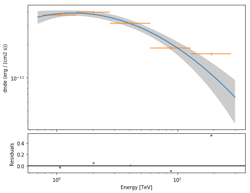
In [7]:
ana.spectrum_result.plot(
    energy_range=ana.fit.fit_range,
    energy_power=2,
    flux_unit='erg-1 cm-2 s-1',
    fig_kwargs=dict(figsize = (8,8)),
)
Out[7]:
(<matplotlib.axes._subplots.AxesSubplot at 0x138228828>,
 <matplotlib.axes._subplots.AxesSubplot at 0x138375c50>)
Exercises
Rerun the analysis, changing some aspects of the analysis as you like:
- only use one or two observations
- a different spectral model
- different config options for the spectral analysis
- different energy binning for the spectral point computation
Observe how the measured spectrum changes.