This is a fixed-text formatted version of a Jupyter notebook

• Try online

• You can contribute with your own notebooks in this GitHub repository.

• Source files: extended_source_spectral_analysis.ipynb | extended_source_spectral_analysis.py

Spectral analysis of extended sources

Prerequisites:

• Understanding of spectral analysis techniques in classical Cherenkov astronomy.

• Understanding of how the spectrum and cube extraction API works, please refer to the spectrum extraction notebook and to the 3D analysis notebook.

Context

Many VHE sources in the Galaxy are extended. Studying them with a 1D spectral analysis is more complex than studying point sources. One often has to use complex (i.e. non circular) regions and more importantly, one has to take into account the fact that the instrument response is non uniform over the selectred region. A typical example is given by the supernova remnant RX J1713-3935 which is nearly 1 degree in diameter. See the following article.

Objective: Measure the spectrum of RX J1713-3945 in a 1 degree region fully enclosing it.

Proposed approach:

We have seen in the general presentation of the spectrum extraction for point sources, see the corresponding notebook, that Gammapy uses specific datasets makers to first produce reduced spectral data and then to extract OFF measurements with reflected background techniques: the gammapy.makers.SpectrumDatasetMaker and the gammapy.makers.ReflectedRegionsBackgroundMaker. The former simply computes the reduced IRF at the center of the ON region (assumed to be circular).

This is no longer valid for extended sources. To be able to compute average responses in the ON region, Gammapy relies on the creation of a cube enclosing it (i.e. a gammapy.datasets.MapDataset) which can be reduced to a simple spectrum (i.e. a gammapy.datasets.SpectrumDataset). We can then proceed with the OFF extraction as the standard point source case.

In summary, we have to:

• Define an ON region (a ~regions.SkyRegion) fully enclosing the source we want to study.

• Define a geometry that fully contains the region and that covers the required energy range (beware in particular, the true energy range).

• Create the necessary makers :

  • the map dataset maker : gammapy.makers.MapDatasetMaker

  • the OFF background maker, here a gammapy.makers.ReflectedRegionsBackgroundMaker

  • and usually the safe range maker : gammapy.makers.SafeRangeMaker

• Perform the data reduction loop. And for every observation:

  • Produce a map dataset and squeeze it to a spectrum dataset with gammapy.datasets.MapDataset.to_spectrum_dataset(on_region)

  • Extract the OFF data to produce a gammapy.datasets.SpectrumDatasetOnOff and compute a safe range for it.

  • Stack or store the resulting spectrum dataset.

• Finally proceed with model fitting on the dataset as usual.

Here, we will use the RX J1713-3945 observations from the H.E.S.S. first public test data release. The tutorial is implemented with the intermediate level API.

Setup

As usual, we’ll start with some general imports…

%matplotlib inline
import matplotlib.pyplot as plt

import astropy.units as u
from astropy.coordinates import SkyCoord, Angle
from regions import CircleSkyRegion
from gammapy.maps import Map, MapAxis, WcsGeom
from gammapy.modeling import Fit
from gammapy.data import DataStore
from gammapy.modeling.models import PowerLawSpectralModel, SkyModel
from gammapy.datasets import Datasets, MapDataset
from gammapy.makers import (
    SafeMaskMaker,
    MapDatasetMaker,
    ReflectedRegionsBackgroundMaker,
)

Select the data

We first set the datastore and retrieve a few observations from our source.

datastore = DataStore.from_dir("$GAMMAPY_DATA/hess-dl3-dr1/")
obs_ids = [20326, 20327, 20349, 20350, 20396, 20397]
# In case you want to use all RX J1713 data in the HESS DR1
# other_ids=[20421, 20422, 20517, 20518, 20519, 20521, 20898, 20899, 20900]

observations = datastore.get_observations(obs_ids)

Prepare the datasets creation

Select the ON region

Here we take a simple 1 degree circular region because it fits well with the morphology of RX J1713-3945. More complex regions could be used e.g. ~regions.EllipseSkyRegion or ~regions.RectangleSkyRegion.

target_position = SkyCoord(347.3, -0.5, unit="deg", frame="galactic")
radius = Angle("0.5 deg")
on_region = CircleSkyRegion(target_position, radius)

Define the geometries

This part is especially important. - We have to define first energy axes. They define the axes of the resulting gammapy.datasets.SpectrumDatasetOnOff. In particular, we have to be careful to the true energy axis: it has to cover a larger range than the reconstructed energy one. - Then we define the geometry itself. It does not need to be very finely binned and should enclose all the ON region. To limit CPU and memory usage, one should avoid using a much larger region.

# The binning of the final spectrum is defined here.
energy_axis = MapAxis.from_energy_bounds(0.3, 40.0, 10, unit="TeV")

# Reduced IRFs are defined in true energy (i.e. not measured energy).
energy_axis_true = MapAxis.from_energy_bounds(
    0.05, 100, 30, unit="TeV", name="energy_true"
)

# Here we use 1.5 degree which is slightly larger than needed.
geom = WcsGeom.create(
    skydir=target_position,
    binsz=0.04,
    width=(1.5, 1.5),
    frame="galactic",
    proj="CAR",
    axes=[energy_axis],
)

Create the makers

First we instantiate the target gammapy.datasets.MapDataset.

stacked = MapDataset.create(
    geom=geom, energy_axis_true=energy_axis_true, name="rxj-stacked"
)

Now we create its associated maker. Here we need to produce, counts, exposure and edisp (energy dispersion) entries. PSF and IRF background are not needed, therefore we don’t compute them.

maker = MapDatasetMaker(selection=["counts", "exposure", "edisp"])

Now we create the OFF background maker for the spectra. If we have an exclusion region, we have to pass it here. We also define the safe range maker.

bkg_maker = ReflectedRegionsBackgroundMaker()
safe_mask_maker = SafeMaskMaker(
    methods=["aeff-default", "aeff-max"], aeff_percent=10
)

Perform the data reduction loop.

We can now run over selected observations. For each of them, we: - create the map dataset and stack it on our target dataset. - squeeze the map dataset to a spectral dataset in the ON region - Compute the OFF and create a gammapy.datasets.SpectrumDatasetOnOff object - Run the safe mask maker on it - Add the gammapy.datasets.SpectrumDatasetOnOff to the list.

%%time
datasets = Datasets()

for obs in observations:
    # A MapDataset is filled in this geometry
    dataset = maker.run(stacked, obs)
    # To make images, the resulting dataset cutout is stacked onto the final one
    stacked.stack(dataset)

    # Extract 1D spectrum
    spectrum_dataset = dataset.to_spectrum_dataset(
        on_region, name=f"obs-{obs.obs_id}"
    )
    # Compute OFF
    spectrum_dataset = bkg_maker.run(spectrum_dataset, obs)
    # Define safe mask
    spectrum_dataset = safe_mask_maker.run(spectrum_dataset, obs)
    # Append dataset to the list
    datasets.append(spectrum_dataset)

CPU times: user 3.15 s, sys: 184 ms, total: 3.34 s
Wall time: 3.37 s

datasets.meta_table

Table length=6

NAME	TYPE	TELESCOP	OBS_ID	RA_PNT	DEC_PNT
				deg	deg
str9	str20	str4	int64	float64	float64
obs-20326	SpectrumDatasetOnOff	HESS	20326	259.29852294921875	-39.76222229003906
obs-20327	SpectrumDatasetOnOff	HESS	20327	257.4773254394531	-39.76222229003906
obs-20349	SpectrumDatasetOnOff	HESS	20349	259.29852294921875	-39.76222229003906
obs-20350	SpectrumDatasetOnOff	HESS	20350	257.4773254394531	-39.76222229003906
obs-20396	SpectrumDatasetOnOff	HESS	20396	258.3879089355469	-39.06222152709961
obs-20397	SpectrumDatasetOnOff	HESS	20397	258.3879089355469	-40.462223052978516

Explore the results

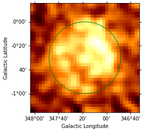
First let’s look at the data to see if our region is correct. We plot it over the excess. To do so we convert it to a pixel region using the WCS information stored on the geom.

stacked.counts.sum_over_axes().smooth(width="0.05 deg").plot()
on_region.to_pixel(stacked.counts.geom.wcs).plot()

<matplotlib.axes._subplots.WCSAxesSubplot at 0x118c803c8>

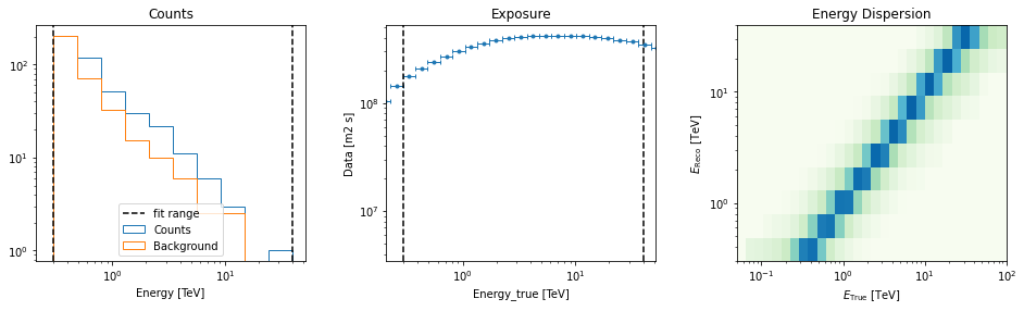
We now turn to the spectral datasets. We can peek at their content:

datasets[0].peek()

(<matplotlib.axes._subplots.AxesSubplot at 0x1190bb7f0>,
 <matplotlib.axes._subplots.AxesSubplot at 0x119208c50>,
 <matplotlib.axes._subplots.AxesSubplot at 0x11d256e80>)

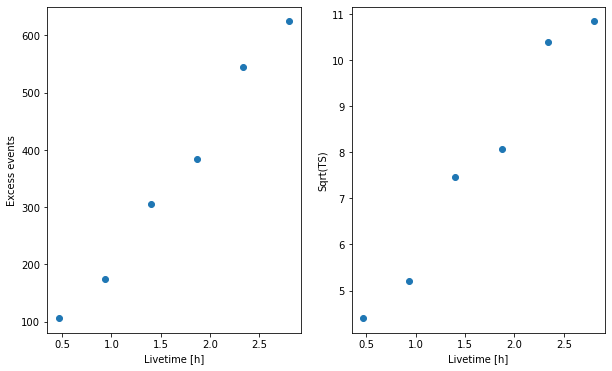
Cumulative excess and signficance

Finally, we can look at cumulative significance and number of excesses. This is done with the info_table method of gammapy.datasets.Datasets.

info_table = datasets.info_table(cumulative=True)

info_table

Table length=6

name	counts	background	excess	sqrt_ts	npred	npred_background	npred_signal	exposure_min	exposure_max	livetime	ontime	counts_rate	background_rate	excess_rate	n_bins	n_fit_bins	stat_type	stat_sum	counts_off	acceptance	acceptance_off	alpha
								m2 s	m2 s	s	s	1 / s	1 / s	1 / s
str9	float32	float64	float64	float64	float64	float64	float64	float64	float64	float64	float64	float64	float64	float64	int64	int64	str5	float64	float32	float64	float64	float64
obs-20326	450.0	343.5	106.5	4.405517626186096	378.99999999999994	378.99999999999994	nan	4309258.042057533	422238157.51238155	1683.0	1683.0	0.26737967914438504	0.20409982174688057	0.06327985739750445	10	10	wstat	41.619587630493804	687.0	10.0	20.0	0.5
obs-20326	845.0	670.5	174.5	5.215405763158092	728.6666666666667	728.6666666666667	nan	14662719.327748926	832059034.478945	3366.0	3366.0	0.2510398098633393	0.19919786096256684	0.05184194890077243	10	10	wstat	68.99758872776455	1341.0	10.0	20.0	0.5
obs-20326	1288.0	983.0	305.0	7.457874883123557	1084.6666666666667	1084.6666666666667	nan	25046841.769557744	1241412951.5114164	5048.0	5048.0	0.2551505546751189	0.19473058637083993	0.06041996830427892	10	10	wstat	110.36192929546934	1966.0	10.0	20.0	0.5
obs-20326	1725.0	1341.0	384.0	8.075257505628382	1468.9999999999998	1468.9999999999998	nan	29517317.73469796	1662189705.5499349	6730.0	6730.0	0.2563150074294205	0.19925705794947995	0.05705794947994056	10	10	wstat	150.00796042782275	2682.0	10.0	20.0	0.5
obs-20326	2198.0	1653.0001220703125	544.9998779296875	10.400166037309209	1823.1466301979633	1823.1466301979633	nan	39224336.77289754	2071146470.3666286	8413.0	8413.0	0.2612623321050755	0.1964816500737326	0.06478068203134286	10	10	wstat	193.54833987070583	3618.0	10.0	21.887475967407227	0.44348058104515076
obs-20326	2626.0	2001.5001220703125	624.4998779296875	10.837684594884903	2198.593368883069	2198.593368883069	nan	41782883.40346215	2500415797.968303	10095.0	10095.0	0.26012877662209016	0.1982664806409423	0.06186229598114785	10	10	wstat	213.44165945794245	4315.0	10.0	21.55883026123047	0.4485357403755188

fig = plt.figure(figsize=(10, 6))
ax = fig.add_subplot(121)
ax.plot(
    info_table["livetime"].to("h"), info_table["excess"], marker="o", ls="none"
)
plt.xlabel("Livetime [h]")
plt.ylabel("Excess events")

ax = fig.add_subplot(122)
ax.plot(
    info_table["livetime"].to("h"),
    info_table["sqrt_ts"],
    marker="o",
    ls="none",
)
plt.xlabel("Livetime [h]")
plt.ylabel("Sqrt(TS)");

Perform spectral model fitting

Here we perform a joint fit.

We first create the model, here a simple powerlaw, and assign it to every dataset in the gammapy.datasets.Datasets.

spectral_model = PowerLawSpectralModel(
    index=2, amplitude=2e-11 * u.Unit("cm-2 s-1 TeV-1"), reference=1 * u.TeV
)
model = SkyModel(spectral_model=spectral_model, name="RXJ 1713")

datasets.models = [model]

Now we can run the fit

fit_joint = Fit(datasets)
result_joint = fit_joint.run()
print(result_joint)

OptimizeResult

        backend    : minuit
        method     : minuit
        success    : True
        message    : Optimization terminated successfully.
        nfev       : 39
        total stat : 72.95

Explore the fit results

First the fitted parameters values and their errors.

result_joint.parameters.to_table()

Table length=3

name	value	unit	min	max	frozen	error
str9	float64	str14	float64	float64	bool	float64
index	2.1021e+00		nan	nan	False	6.657e-02
amplitude	1.2869e-11	cm-2 s-1 TeV-1	nan	nan	False	1.023e-12
reference	1.0000e+00	TeV	nan	nan	True	0.000e+00

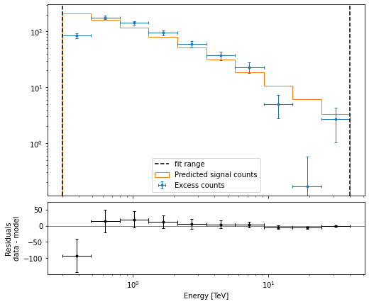
Then plot the fit result to compare measured and expected counts. Rather than plotting them for each individual dataset, we stack all datasets and plot the fit result on the result.

# First stack them all
reduced = datasets.stack_reduce()
# Assign the fitted model
reduced.models = model
# Plot the result
reduced.plot_fit();