This is a fixed-text formatted version of a Jupyter notebook

• Try online
• You can contribute with your own notebooks in this GitHub repository.
• Source files: light_curve.ipynb | light_curve.py

Light curve estimation

Introduction

This tutorial presents a new light curve estimator that works with dataset objects. We will demonstrate how to compute a light curve from 3D data cubes as well as 1D spectral data using the MapDataset, SpectrumDatasetOnOff and LightCurveEstimator classes.

We will use the four Crab nebula observations from the H.E.S.S. first public test data release and compute per-observation fluxes. The Crab nebula is not known to be variable at TeV energies, so we expect constant brightness within statistical and systematic errors.

The main classes we will use are:

• gammapy.time.LightCurve
• gammapy.time.LightCurveEstimator

Setup

As usual, we’ll start with some general imports…

%matplotlib inline
import matplotlib.pyplot as plt

import astropy.units as u
from astropy.coordinates import SkyCoord
from astropy.time import Time
import logging

log = logging.getLogger(__name__)

Now let’s import gammapy specific classes and functions

from gammapy.data import ObservationFilter, DataStore
from gammapy.spectrum.models import PowerLaw
from gammapy.image.models import SkyPointSource
from gammapy.cube.models import SkyModel, BackgroundModel
from gammapy.cube import PSFKernel, MapMaker, MapDataset
from gammapy.maps import WcsGeom, MapAxis
from gammapy.irf import make_mean_psf, make_mean_edisp
from gammapy.time import LightCurveEstimator

Select the data

We look for relevant observations in the datastore.

data_store = DataStore.from_file(
    "$GAMMAPY_DATA/hess-dl3-dr1/hess-dl3-dr3-with-background.fits.gz"
)
mask = data_store.obs_table["TARGET_NAME"] == "Crab"
obs_ids = data_store.obs_table["OBS_ID"][mask].data
crab_obs = data_store.get_observations(obs_ids)

Define time intervals

We create a list of time intervals. Here we use one time bin per observation.

time_intervals = [(obs.tstart, obs.tstop) for obs in crab_obs]

3D data reduction

Define the analysis geometry

Here we define the geometry used in the analysis. We use the same WCS map structure but we use two different binnings for reco and true energy axes. This allows for a broader coverage of the response.

# Target definition
target_position = SkyCoord(ra=83.63308, dec=22.01450, unit="deg")

# Define geoms
emin, emax = [0.7, 10] * u.TeV
energy_axis = MapAxis.from_bounds(
    emin.value, emax.value, 10, unit="TeV", name="energy", interp="log"
)
geom = WcsGeom.create(
    skydir=target_position,
    binsz=0.04,
    width=(2, 2),
    coordsys="CEL",
    proj="CAR",
    axes=[energy_axis],
)

etrue_axis = MapAxis.from_bounds(
    0.1, 20, 20, unit="TeV", name="energy", interp="log"
)

geom_true = WcsGeom.create(
    skydir=target_position,
    binsz=0.04,
    width=(2, 2),
    coordsys="CEL",
    proj="CAR",
    axes=[etrue_axis],
)

Define the 3D model

The light curve is based on a 3D fit of a map dataset in time bins. We therefore need to define the source model to be applied. Here a point source with power law spectrum. We freeze its parameters assuming they were previously extracted

# Define the source model - Use a pointsource + integrated power law model to directly get flux

spatial_model = SkyPointSource(
    lon_0=target_position.ra, lat_0=target_position.dec, frame="icrs"
)

spectral_model = PowerLaw(
    index=2.6,
    amplitude=2.0e-11 * u.Unit("1 / (cm2 s TeV)"),
    reference=1 * u.TeV,
)
spectral_model.parameters["index"].frozen = False

sky_model = SkyModel(
    spatial_model=spatial_model, spectral_model=spectral_model, name=""
)
sky_model.parameters["lon_0"].frozen = True
sky_model.parameters["lat_0"].frozen = True

Make the map datasets

The following function is in charge of the MapDataset production. It will later be fully covered in the data reduction chain

# psf_kernel and MapMaker for each segment
def make_map_dataset(
    observations, target_pos, geom, geom_true, offset_max=2 * u.deg
):
    maker = MapMaker(geom, offset_max, geom_true=geom_true)
    maps = maker.run(observations)
    table_psf = make_mean_psf(observations, target_pos)

    # PSF kernel used for the model convolution
    psf_kernel = PSFKernel.from_table_psf(
        table_psf, geom_true, max_radius="0.3 deg"
    )
    edisp = make_mean_edisp(
        observations,
        target_pos,
        e_true=geom_true.axes[0].edges,
        e_reco=geom.axes[0].edges,
    )
    background_model = BackgroundModel(maps["background"])
    background_model.parameters["norm"].frozen = False
    background_model.parameters["tilt"].frozen = True

    dataset = MapDataset(
        counts=maps["counts"],
        exposure=maps["exposure"],
        background_model=background_model,
        psf=psf_kernel,
        edisp=edisp,
    )
    return dataset

Now we perform the actual data reduction in time bins

%%time

datasets = []

for time_interval in time_intervals:
    # get filtered observation lists in time interval
    obs = crab_obs.select_time(time_interval)
    # Proceed with further analysis only if there are observations
    # in the selected time window
    if len(obs) == 0:
        log.warning(
            "No observations found in time interval:"
            "{t_min} - {t_max}".format(
                t_min=time_interval[0], t_max=time_interval[1]
            )
        )
        continue
    dataset = make_map_dataset(obs, target_position, geom, geom_true)
    dataset.counts.meta["t_start"] = time_interval[0]
    dataset.counts.meta["t_stop"] = time_interval[1]
    datasets.append(dataset)

CPU times: user 2.92 s, sys: 152 ms, total: 3.07 s
Wall time: 3.07 s

Light Curve estimation: the 3D case

Now that we have created the datasets we assign them the model to be fitted:

for dataset in datasets:
    # Copy the source model
    model = sky_model.copy(name="crab")
    dataset.model = model

We can now create the light curve estimator by passing it the list of datasets. We can optionally ask for parameters reoptimization during fit, e.g. to fit background normalization in each time bin.

lc_maker = LightCurveEstimator(datasets, source="crab", reoptimize=True)

We now run the estimator once we pass it the energy interval on which to compute the integral flux of the source.

%%time
lc = lc_maker.run(e_ref=1 * u.TeV, e_min=1.0 * u.TeV, e_max=10.0 * u.TeV)

CPU times: user 14.8 s, sys: 222 ms, total: 15.1 s
Wall time: 15.1 s

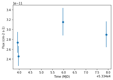
The LightCurve object contains a table which we can explore.

lc.table["time_min", "time_max", "flux", "flux_err"]

Table length=4

time_min	time_max	flux	flux_err
		1 / (cm2 s)	1 / (cm2 s)
float64	float64	float64	float64
53343.92234009259	53343.94186555556	2.7339067197215866e-11	2.100460186805052e-12
53343.95421509259	53343.97369425926	2.4575209334948127e-11	2.027293009588302e-12
53345.96198129629	53345.98149518518	3.147648428762074e-11	2.783720854376958e-12
53347.913196574074	53347.93271046296	2.8951354849167565e-11	2.626377535137574e-12

We finally plot the light curve

lc.plot(marker="o")

<matplotlib.axes._subplots.AxesSubplot at 0x1272a2f60>

Performing the same analysis with 1D spectra

First the relevant imports

We import the missing classes for spectral data reduction

from regions import CircleSkyRegion
from astropy.coordinates import Angle

from gammapy.background import ReflectedRegionsBackgroundEstimator
from gammapy.spectrum import SpectrumExtraction

Defining the geometry

We need to define the ON extraction region. We will keep the same reco and true energy axes as in 3D.

# Target definition
on_region_radius = Angle("0.11 deg")
on_region = CircleSkyRegion(center=target_position, radius=on_region_radius)

Extracting the background

We perform here an ON - OFF measurement with reflected regions. We perform first the background extraction.

bkg_estimator = ReflectedRegionsBackgroundEstimator(
    on_region=on_region, observations=crab_obs
)
bkg_estimator.run()

Creation of the datasets

We now apply spectral extraction to create the datasets.

NB: we are using here time intervals defined by the observations start and stop times. The standard observation based spectral extraction is therefore defined in the right time bins.

A proper time resolved spectral extraction will be included in a coming gammapy release.

# Note that we are not performing the extraction in time bins
extraction = SpectrumExtraction(
    observations=crab_obs,
    bkg_estimate=bkg_estimator.result,
    containment_correction=True,
    e_reco=energy_axis.edges,
    e_true=etrue_axis.edges,
)
extraction.run()
datasets_1d = extraction.spectrum_observations

# we need to set the times manually for now
for dataset, time_interval in zip(datasets_1d, time_intervals):
    dataset.counts.meta = dict()
    dataset.counts.meta["t_start"] = time_interval[0]
    dataset.counts.meta["t_stop"] = time_interval[1]

/Users/adonath/github/adonath/gammapy/gammapy/spectrum/extract.py:232: RuntimeWarning: invalid value encountered in true_divide
  self.containment = new_aeff.data.data.value / self._aeff.data.data.value

Light Curve estimation for 1D spectra

Now that we’ve reduced the 1D data we assign again the model to the datasets

for dataset in datasets_1d:
    # Copy the source model
    model = spectral_model.copy()
    model.name = "crab"
    dataset.model = model

We can now call the LightCurveEstimator in a perfectly identical manner.

lc_maker_1d = LightCurveEstimator(datasets_1d, source="crab", reoptimize=False)

%%time
lc_1d = lc_maker_1d.run(e_ref=1 * u.TeV, e_min=1.0 * u.TeV, e_max=10.0 * u.TeV)

CPU times: user 215 ms, sys: 2.13 ms, total: 217 ms
Wall time: 215 ms

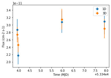
Compare results

Finally we compare the result for the 1D and 3D lightcurve in a single figure:

ax = lc_1d.plot(marker="o", label="1D")
lc.plot(ax=ax, marker="o", label="3D")
plt.legend()

<matplotlib.legend.Legend at 0x1265650f0>