This is a fixed-text formatted version of a Jupyter notebook
Try online

You can contribute with your own notebooks in this GitHub repository.
Source files: simulate_3d.ipynb | simulate_3d.py
3D simulation and fitting
Prerequisites
Knowledge of 3D extraction and datasets used in gammapy, see for instance the first analysis tutorial
Context
To simulate a specific observation, it is not always necessary to simulate the full photon list. For many uses cases, simulating directly a reduced binned dataset is enough: the IRFs reduced in the correct geometry are combined with a source model to predict an actual number of counts per bin. The latter is then used to simulate a reduced dataset using Poisson probability distribution.
This can be done to check the feasibility of a measurement (performance / sensitivity study), to test whether fitted parameters really provide a good fit to the data etc.
Here we will see how to perform a 3D simulation of a CTA observation, assuming both the spectral and spatial morphology of an observed source.
Objective: simulate a 3D observation of a source with CTA using the CTA 1DC response and fit it with the assumed source model.
Proposed approach:
Here we can’t use the regular observation objects that are connected to a DataStore. Instead we will create a fake gammapy.data.Observation that contain some pointing information and the CTA 1DC IRFs (that are loaded with gammapy.irf.load_cta_irfs).
Then we will create a gammapy.datasets.MapDataset geometry and create it with the gammapy.makers.MapDatasetMaker.
Then we will be able to define a model consisting of a gammapy.modeling.models.PowerLawSpectralModel and a gammapy.modeling.models.GaussianSpatialModel. We will assign it to the dataset and fake the count data.
Imports and versions
[1]:
%matplotlib inline
[2]:
import numpy as np
import astropy.units as u
from astropy.coordinates import SkyCoord
from gammapy.irf import load_cta_irfs
from gammapy.maps import WcsGeom, MapAxis
from gammapy.modeling.models import (
    PowerLawSpectralModel,
    GaussianSpatialModel,
    SkyModel,
    Models,
    FoVBackgroundModel,
)
from gammapy.makers import MapDatasetMaker, SafeMaskMaker
from gammapy.modeling import Fit
from gammapy.data import Observation
from gammapy.datasets import MapDataset
[3]:
!gammapy info --no-envvar --no-dependencies --no-system
Gammapy package:

        version                : 0.18.1
        path                   : /Users/adonath/github/adonath/gammapy/gammapy
Simulation
We will simulate using the CTA-1DC IRFs shipped with gammapy. Note that for dedictaed CTA simulations, you can simply use `Observation.from_caldb() <>`__ without having to externally load the IRFs
[4]:
# Loading IRFs
irfs = load_cta_irfs(
    "$GAMMAPY_DATA/cta-1dc/caldb/data/cta/1dc/bcf/South_z20_50h/irf_file.fits"
)
Invalid unit found in background table! Assuming (s-1 MeV-1 sr-1)
[5]:
# Define the observation parameters (typically the observation duration and the pointing position):
livetime = 2.0 * u.hr
pointing = SkyCoord(0, 0, unit="deg", frame="galactic")
[6]:
# Define map geometry for binned simulation
energy_reco = MapAxis.from_edges(
    np.logspace(-1.0, 1.0, 10), unit="TeV", name="energy", interp="log"
)
geom = WcsGeom.create(
    skydir=(0, 0),
    binsz=0.02,
    width=(6, 6),
    frame="galactic",
    axes=[energy_reco],
)
# It is usually useful to have a separate binning for the true energy axis
energy_true = MapAxis.from_edges(
    np.logspace(-1.5, 1.5, 30), unit="TeV", name="energy", interp="log"
)

empty = MapDataset.create(geom, name="dataset-simu")
[7]:
# Define sky model to used simulate the data.
# Here we use a Gaussian spatial model and a Power Law spectral model.
spatial_model = GaussianSpatialModel(
    lon_0="0.2 deg", lat_0="0.1 deg", sigma="0.3 deg", frame="galactic"
)
spectral_model = PowerLawSpectralModel(
    index=3, amplitude="1e-11 cm-2 s-1 TeV-1", reference="1 TeV"
)
model_simu = SkyModel(
    spatial_model=spatial_model,
    spectral_model=spectral_model,
    name="model-simu",
)

bkg_model = FoVBackgroundModel(dataset_name="dataset-simu")

models = Models([model_simu, bkg_model])
print(models)
Models

Component 0: SkyModel

  Name                      : model-simu
  Datasets names            : None
  Spectral model type       : PowerLawSpectralModel
  Spatial  model type       : GaussianSpatialModel
  Temporal model type       :
  Parameters:
    index                   :   3.000
    amplitude               :   1.00e-11  1 / (cm2 s TeV)
    reference    (frozen)   :   1.000  TeV
    lon_0                   :   0.200  deg
    lat_0                   :   0.100  deg
    sigma                   :   0.300  deg
    e            (frozen)   :   0.000
    phi          (frozen)   :   0.000  deg

Component 1: FoVBackgroundModel

  Name                      : dataset-simu-bkg
  Datasets names            : ['dataset-simu']
  Spectral model type       : PowerLawNormSpectralModel
  Parameters:
    norm                    :   1.000
    tilt         (frozen)   :   0.000
    reference    (frozen)   :   1.000  TeV
Now, comes the main part of dataset simulation. We create an in-memory observation and an empty dataset. We then predict the number of counts for the given model, and Poission fluctuate it using fake() to make a simulated counts maps. Keep in mind that it is important to specify the selection of the maps that you want to produce
[8]:
# Create an in-memory observation
obs = Observation.create(pointing=pointing, livetime=livetime, irfs=irfs)
print(obs)
Observation

        obs id            : 0
        tstart            : 51544.00
        tstop             : 51544.08
        duration          : 7200.00 s
        pointing (icrs)   : 266.4 deg, -28.9 deg

        deadtime fraction : 0.0%
[9]:
# Make the MapDataset
maker = MapDatasetMaker(selection=["exposure", "background", "psf", "edisp"])

maker_safe_mask = SafeMaskMaker(methods=["offset-max"], offset_max=4.0 * u.deg)

dataset = maker.run(empty, obs)
dataset = maker_safe_mask.run(dataset, obs)
print(dataset)
MapDataset
----------

  Name                            : dataset-simu

  Total counts                    : nan
  Total background counts         : 161250.95
  Total excess counts             : nan

  Predicted counts                : 161250.95
  Predicted background counts     : 161250.95
  Predicted excess counts         : nan

  Exposure min                    : 6.41e+07 m2 s
  Exposure max                    : 2.53e+10 m2 s

  Number of total bins            : 0
  Number of fit bins              : 804492

  Fit statistic type              : cash
  Fit statistic value (-2 log(L)) : nan

  Number of models                : 0
  Number of parameters            : 0
  Number of free parameters       : 0
[10]:
# Add the model on the dataset and Poission fluctuate
dataset.models = models
dataset.fake()
# Do a print on the dataset - there is now a counts maps
print(dataset)
MapDataset
----------

  Name                            : dataset-simu

  Total counts                    : 169978
  Total background counts         : 161250.95
  Total excess counts             : 8727.05

  Predicted counts                : 169690.08
  Predicted background counts     : 161250.95
  Predicted excess counts         : 8439.14

  Exposure min                    : 6.41e+07 m2 s
  Exposure max                    : 2.53e+10 m2 s

  Number of total bins            : 810000
  Number of fit bins              : 804492

  Fit statistic type              : cash
  Fit statistic value (-2 log(L)) : 565057.78

  Number of models                : 2
  Number of parameters            : 11
  Number of free parameters       : 6

  Component 0: SkyModel

    Name                      : model-simu
    Datasets names            : None
    Spectral model type       : PowerLawSpectralModel
    Spatial  model type       : GaussianSpatialModel
    Temporal model type       :
    Parameters:
      index                   :   3.000
      amplitude               :   1.00e-11  1 / (cm2 s TeV)
      reference    (frozen)   :   1.000  TeV
      lon_0                   :   0.200  deg
      lat_0                   :   0.100  deg
      sigma                   :   0.300  deg
      e            (frozen)   :   0.000
      phi          (frozen)   :   0.000  deg

  Component 1: FoVBackgroundModel

    Name                      : dataset-simu-bkg
    Datasets names            : ['dataset-simu']
    Spectral model type       : PowerLawNormSpectralModel
    Parameters:
      norm                    :   1.000
      tilt         (frozen)   :   0.000
      reference    (frozen)   :   1.000  TeV
Now use this dataset as you would in all standard analysis. You can plot the maps, or proceed with your custom analysis. In the next section, we show the standard 3D fitting as in analysis_3d.
[11]:
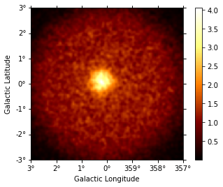
# To plot, eg, counts:
dataset.counts.smooth(0.05 * u.deg).plot_interactive(
    add_cbar=True, stretch="linear"
)
Fit
In this section, we do a usual 3D fit with the same model used to simulated the data and see the stability of the simulations. Often, it is useful to simulate many such datasets and look at the distribution of the reconstructed parameters.
[12]:
models_fit = models.copy()
[13]:
# We do not want to fit the background in this case, so we will freeze the parameters
models_fit["dataset-simu-bkg"].spectral_model.norm.frozen = True
models_fit["dataset-simu-bkg"].spectral_model.tilt.frozen = True
[14]:
dataset.models = models_fit
print(dataset.models)
DatasetModels

Component 0: SkyModel

  Name                      : model-simu
  Datasets names            : None
  Spectral model type       : PowerLawSpectralModel
  Spatial  model type       : GaussianSpatialModel
  Temporal model type       :
  Parameters:
    index                   :   3.000
    amplitude               :   1.00e-11  1 / (cm2 s TeV)
    reference    (frozen)   :   1.000  TeV
    lon_0                   :   0.200  deg
    lat_0                   :   0.100  deg
    sigma                   :   0.300  deg
    e            (frozen)   :   0.000
    phi          (frozen)   :   0.000  deg

Component 1: FoVBackgroundModel

  Name                      : dataset-simu-bkg
  Datasets names            : ['dataset-simu']
  Spectral model type       : PowerLawNormSpectralModel
  Parameters:
    norm         (frozen)   :   1.000
    tilt         (frozen)   :   0.000
    reference    (frozen)   :   1.000  TeV
[15]:
%%time
fit = Fit([dataset])
result = fit.run(optimize_opts={"print_level": 1})
------------------------------------------------------------------
| FCN = 5.651e+05               |     Ncalls=129 (129 total)     |
| EDM = 8.83e-06 (Goal: 0.0002) |            up = 1.0            |
------------------------------------------------------------------
|  Valid Min.   | Valid Param.  | Above EDM | Reached call limit |
------------------------------------------------------------------
|     True      |     True      |   False   |       False        |
------------------------------------------------------------------
| Hesse failed  |   Has cov.    | Accurate  | Pos. def. | Forced |
------------------------------------------------------------------
|     False     |     True      |   True    |   True    | False  |
------------------------------------------------------------------
CPU times: user 5.6 s, sys: 342 ms, total: 5.94 s
Wall time: 6 s
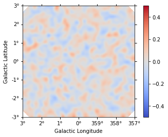
[16]:
dataset.plot_residuals_spatial(method="diff/sqrt(model)", vmin=-0.5, vmax=0.5)
[16]:
<matplotlib.axes._subplots.WCSAxesSubplot at 0x1152e70f0>
Compare the injected and fitted models:
[17]:
print(
    "True model: \n",
    model_simu,
    "\n\n Fitted model: \n",
    models_fit["model-simu"],
)
True model:
 SkyModel

  Name                      : model-simu
  Datasets names            : None
  Spectral model type       : PowerLawSpectralModel
  Spatial  model type       : GaussianSpatialModel
  Temporal model type       :
  Parameters:
    index                   :   3.000
    amplitude               :   1.00e-11  1 / (cm2 s TeV)
    reference    (frozen)   :   1.000  TeV
    lon_0                   :   0.200  deg
    lat_0                   :   0.100  deg
    sigma                   :   0.300  deg
    e            (frozen)   :   0.000
    phi          (frozen)   :   0.000  deg


 Fitted model:
 SkyModel

  Name                      : model-simu
  Datasets names            : None
  Spectral model type       : PowerLawSpectralModel
  Spatial  model type       : GaussianSpatialModel
  Temporal model type       :
  Parameters:
    index                   :   3.017
    amplitude               :   9.69e-12  1 / (cm2 s TeV)
    reference    (frozen)   :   1.000  TeV
    lon_0                   :   0.205  deg
    lat_0                   :   0.101  deg
    sigma                   :   0.298  deg
    e            (frozen)   :   0.000
    phi          (frozen)   :   0.000  deg
Get the errors on the fitted parameters from the parameter table
[18]:
result.parameters.to_table()
[18]:
| name | value | unit | min | max | frozen | error |
|---|---|---|---|---|---|---|
| str9 | float64 | str14 | float64 | float64 | bool | float64 |
| index | 3.0175e+00 | nan | nan | False | 2.037e-02 | |
| amplitude | 9.6860e-12 | cm-2 s-1 TeV-1 | nan | nan | False | 3.290e-13 |
| reference | 1.0000e+00 | TeV | nan | nan | True | 0.000e+00 |
| lon_0 | 2.0456e-01 | deg | nan | nan | False | 5.887e-03 |
| lat_0 | 1.0071e-01 | deg | -9.000e+01 | 9.000e+01 | False | 5.927e-03 |
| sigma | 2.9817e-01 | deg | 0.000e+00 | nan | False | 4.057e-03 |
| e | 0.0000e+00 | 0.000e+00 | 1.000e+00 | True | 0.000e+00 | |
| phi | 0.0000e+00 | deg | nan | nan | True | 0.000e+00 |
| norm | 1.0000e+00 | nan | nan | True | 0.000e+00 | |
| tilt | 0.0000e+00 | nan | nan | True | 0.000e+00 | |
| reference | 1.0000e+00 | TeV | nan | nan | True | 0.000e+00 |
[ ]: