Datasets (DL4)#

The gammapy.datasets sub-package contains classes to handle reduced gamma-ray data for modeling and fitting.

The Dataset class bundles reduced data, IRFs and model to perform likelihood fitting and joint-likelihood fitting. All datasets contain a Models container with one or more SkyModel objects that represent additive emission components.

To model and fit data in Gammapy, you have to create a Datasets container object with one or multiple Dataset objects.

Types of supported datasets#

Gammapy has built-in support to create and analyse the following datasets:

Dataset Type	Data Type	Reduced IRFs	Geometry	Additional Quantities	Fit Statistic
`MapDataset`	`counts`	`background`, `psf`, `edisp`, `exposure`,	`WcsGeom` or `RegionGeom`		`cash`
`MapDatasetOnOff`	`counts`	`psf`, `edisp`, `exposure`	`WcsGeom`	`acceptance`, `acceptance_off`, `counts_off`	`wstat`
`SpectrumDataset`	`counts`	`background`, `edisp`, `exposure`	`RegionGeom`		`cash`
`SpectrumDatasetOnOff`	`counts`	`edisp`, `exposure`	`RegionGeom`	`acceptance`, `acceptance_off`, `counts_off`	`wstat`
`FluxPointsDataset`	`flux`	None	None		`chi2`

In addition to the above quantities, a dataset can optionally have a meta_table serialised, which can contain relevant information about the observations used to create the dataset. In general, OnOff datasets should be used when the background is estimated from real off counts, rather than from a background model. The FluxPointsDataset is used to fit pre-computed flux points when no convolution with IRFs are needed.

The map datasets represent 3D cubes (WcsNDMap objects) with two spatial and one energy axis. For 2D images the same map objects and map datasets are used, an energy axis is present but only has one energy bin.

The spectrum datasets represent 1D spectra (RegionNDMap objects) with an energy axis. There are no spatial axes or information, the 1D spectra are obtained for a given on region.

Note that in Gammapy, 2D image analyses are done with 3D cubes with a single energy bin, e.g. for modeling and fitting.

To analyse multiple runs, you can either stack the datasets together, or perform a joint fit across multiple datasets.

Predicted counts#

The total number of predicted counts from a MapDataset are computed per bin like:

\[N_{Pred} = N_{Bkg} + \sum_{Src} N_{Src}\]

Where \(N_{Bkg}\) is the expected counts from the residual hadronic background model and \(N_{Src}\) the predicted counts from a given source model component. The predicted counts from the hadronic background are computed directly from the model in reconstructed energy and spatial coordinates, while the predicted counts from a source are obtained by forward folding with the instrument response:

\[N_{Src} = \mathrm{PSF_{Src}} \circledast \mathrm{EDISP_{Src}}(\mathcal{E} \cdot F_{Src}(l, b, E_{True}))\]

Where \(F_{Src}\) is the integrated flux of the source model, \(\mathcal{E}\) the exposure, \(\mathrm{EDISP}\) the energy dispersion matrix and \(\mathrm{PSF}\) the PSF convolution kernel. The corresponding IRFs are extracted at the current position of the model component defined by \((l, b)\) and assumed to be constant across the size of the source. The detailed expressions to compute the predicted number of counts from a source and corresponding IRFs are given in IRF Theory.

Stacking Multiple Datasets#

Stacking datasets implies that the counts, background and reduced IRFs from all the runs are binned together to get one final dataset for which a likelihood is computed during the fit. Stacking is often useful to reduce the computation effort while analysing multiple runs.

The following table lists how the individual quantities are handled during stacking. Here, \(k\) denotes a bin in reconstructed energy, \(l\) a bin in true energy and \(j\) is the dataset number

Dataset attribute	Behaviour	Implementation
`livetime`	Sum of individual livetimes	\(\overline{t} = \sum_j t_j\)
`mask_safe`	True if the pixel is included in the safe data range.	\(\overline{\epsilon_k} = \sum_{j} \epsilon_{jk}\)
`mask_fit`	Dropped
`counts`	Summed in the data range defined by `mask_safe`	\(\overline{\mathrm{counts}_k} = \sum_j \mathrm{counts}_{jk} \cdot \epsilon_{jk}\)
`background`	Summed in the data range defined by `mask_safe`	\(\overline{\mathrm{bkg}_k} = \sum_j \mathrm{bkg}_{jk} \cdot \epsilon_{jk}\)
`exposure`	Summed in the data range defined by `mask_safe`	\(\overline{\mathrm{exposure}_l} = \sum_{j} \mathrm{exposure}_{jl} \cdot \sum_k \epsilon_{jk}\)
`psf`	Exposure weighted average	\(\overline{\mathrm{psf}_l} = \frac{\sum_{j} \mathrm{psf}_{jl} \cdot \mathrm{exposure}_{jl}} {\sum_{j} \mathrm{exposure}_{jl}}\)
`edisp`	Exposure weighted average, with mask on reconstructed energy	\(\overline{\mathrm{edisp}_{kl}} = \frac{\sum_{j}\mathrm{edisp}_{jkl} \cdot \epsilon_{jk} \cdot \mathrm{exposure}_{jl}} {\sum_{j} \mathrm{exposure}_{jl}}\)
`gti`	Union of individual `gti`

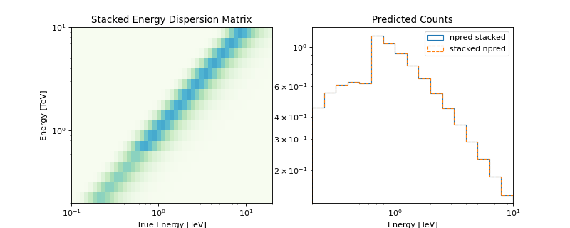
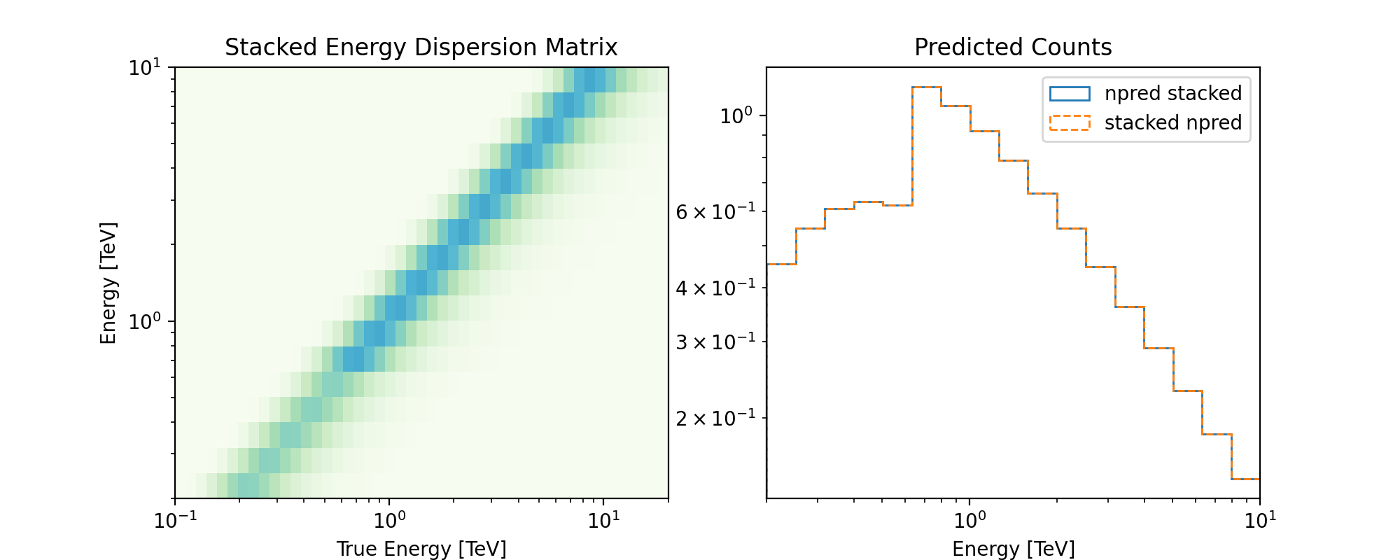
For the model evaluation, an important factor that needs to be accounted for is that the energy threshold changes between observations. With the above implementation using a EDispersionMap, the npred is conserved, ie, the predicted number of counts on the stacked dataset is the sum expected by stacking the npred of the individual runs,

The following plot illustrates the stacked energy dispersion kernel and summed predicted counts for individual as well as stacked spectral datasets:

(png, hires.png, pdf)

Note

A stacked analysis is reasonable only when adding runs taken by the same instrument.
Stacking happens in-place, ie, dataset1.stack(dataset2) will overwrite dataset1
To properly handle masks, it is necessary to stack onto an empty dataset.
Stacking only works for maps with equivalent geometry. Two geometries are called equivalent if one is exactly the same as or can be obtained from a cutout of the other.

Joint Analysis#

An alternative to stacking datasets is a joint fit across all the datasets. For a definition, see Glossary.

The total fit statistic of datasets is the sum of the fit statistic of each dataset. Note that this is not equal to the stacked fit statistic.

A joint fit usually allows a better modeling of the background because the background model parameters can be fit for each dataset simultaneously with the source models. However, a joint fit is, performance wise, very computationally intensive. The fit convergence time increases non-linearly with the number of datasets to be fit. Moreover, depending upon the number of parameters in the background model, even fit convergence might be an issue for a large number of datasets.

To strike a balance, what might be a practical solution for analysis of many runs is to stack runs taken under similar conditions and then do a joint fit on the stacked datasets.

Serialisation of datasets#

The various Map objects contained in MapDataset and MapDatasetOnOff are serialised according to GADF Sky Maps. A hdulist is created with the different attributes, and each of these are written with the data contained in a BinTableHDU with a WcsGeom and a BANDS HDU specifying the non-spatial dimensions. Optionally, a meta_table is also written as an astropy.table.Table containing various information about the observations which created the dataset. While the meta_table can contain useful information for later stage analysis, it is not used anywhere internally within gammapy.

SpectrumDataset follows a similar convention as for MapDataset, but uses a RegionGeom. The region definition follows the standard FITS format, as described here. SpectrumDatasetOnOff can be serialised either according to the above specification, or (by default), according to the OGIP standards.

FluxPointsDatasets are serialised as gammapy.estimators.FluxPoints objects, which contains a set of gammapy.maps.Map objects storing the estimated flux as function of energy, and some optional quantities like typically errors, upper limits, etc. It also contains a reference model, serialised as a TemplateSpectralModel.

Using gammapy.datasets#

Gammapy tutorial notebooks that show how to use this package:

Datasets - Reduced data, IRFs, models

Modelling

Flux point fitting