Getting started#
Installation#
Working with conda?
Gammapy can be installed with Anaconda or Miniconda:
$ conda install -c conda-forge gammapy
Prefer pip?
Gammapy can be installed via pip from PyPI.
$ pip install gammapy
In-depth instructions?
Update existing version? Working with virtual environments? Installing a specific version? Check the advanced installation page.
Quickstart Setup#
The best way to get started and learn Gammapy are the Tutorials. For convenience we provide a pre-defined conda environment file, so you can get additional useful packages together with Gammapy in a virtual isolated environment. First install Miniconda and then just execute the following commands in the terminal:
$ curl -O https://gammapy.org/download/install/gammapy-0.20.1-environment.yml
$ conda env create -f gammapy-0.20.1-environment.yml
Note
On Windows, you have to open up the conda environment file and delete the
lines with sherpa and healpy. Those are optional dependencies that
currently aren’t available on Windows.
Once the environment has been created you can activate it using:
$ conda activate gammapy-0.20.1
You can now proceed to download the Gammapy tutorial notebooks and the example datasets. The total size to download is ~180 MB. Select the location where you want to install the datasets and proceed with the following commands:
$ gammapy download notebooks --release 0.20.1
$ gammapy download datasets
$ export GAMMAPY_DATA=$PWD/gammapy-datasets
You might want to put the definition of the $GAMMAPY_DATA environment
variable in your shell profile setup file that is executed when you open a new
terminal (for example $HOME/.bash_profile).
Note
If you are not using the bash shell, handling of shell environment variables
might be different, e.g. in some shells the command to use is set or something
else instead of export, and also the profile setup file will be different.
On Windows, you should set the GAMMAPY_DATA environment variable in the
“Environment Variables” settings dialog, as explained e.g.
here
Finally start a notebook server by executing:
$ cd notebooks
$ jupyter notebook
If you are new to conda, Python and Jupyter, maybe also read the Using Gammapy guide. If you encountered any issues you can check the Troubleshooting guide.
Tutorials Overview#
Gammapy can read and access data from multiple gamma-ray instruments. Data from
Imaging Atmospheric Cherenkov Telescopes, such as CTA, H.E.S.S., MAGIC
and VERITAS, is typically accessed from the event list data level, called “DL3”.
This is most easily done using the DataStore class. In addition data
can also be accessed from the level of binned events and pre-reduced instrument response functions,
so called “DL4”. This is typically the case for Fermi-LAT data or data from
Water Cherenkov Observatories. This data can be read directly using the
Map and IRFMap classes.
CTA data tutorial HESS data tutorial Fermi-LAT data tutorial
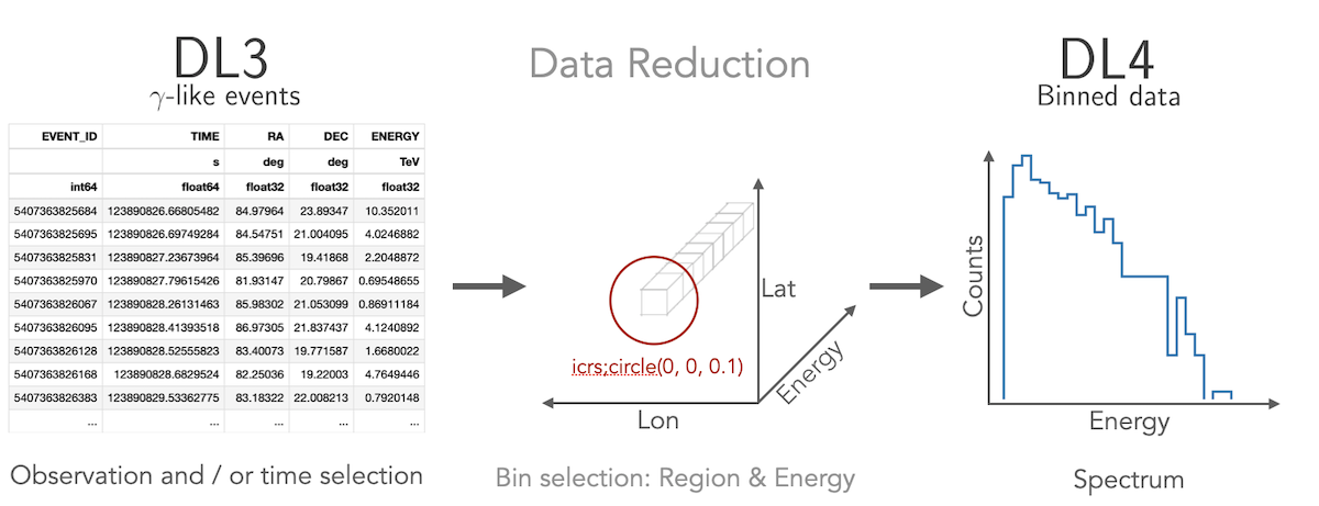
Gammapy lets you create a 1D spectrum by defining an analysis region in
the sky and energy binning using RegionGeom object.
The events and instrument response are binned into RegionNDMap
and IRFMap objects. In addition you can choose to estimate
the background from data using e.g. a reflected regions method.
Flux points can be computed using the FluxPointsEstimator.
1D analysis tutorial 1D analysis tutorial with point-like IRFs 1D analysis tutorial of extended sources
Gammapy treats 2D maps as 3D cubes with one bin in energy. Computation of 2D images can be done following a 3D analysis with one bin with a fixed spectral index, or following the classical ring background estimation.
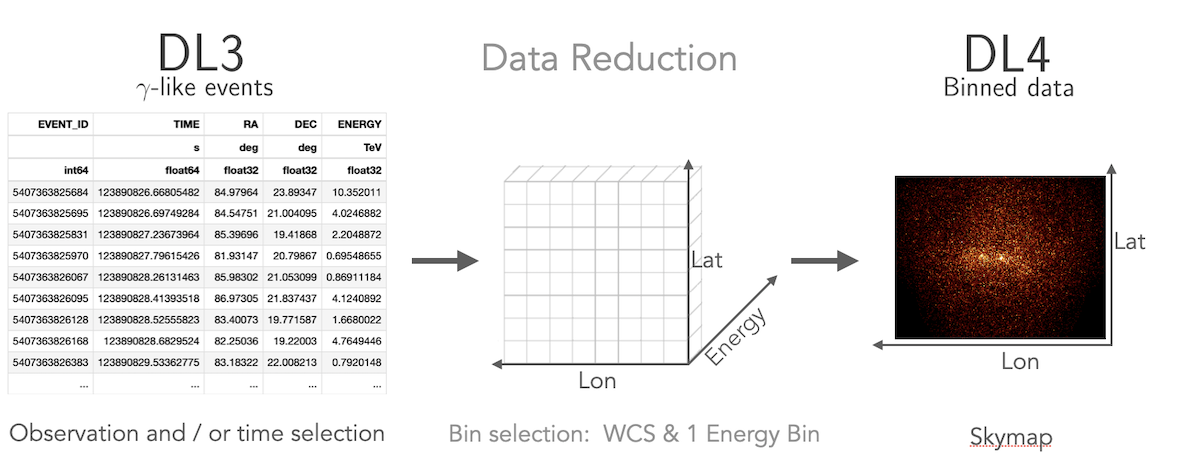
2D analysis tutorial 2D analysis tutorial with ring background
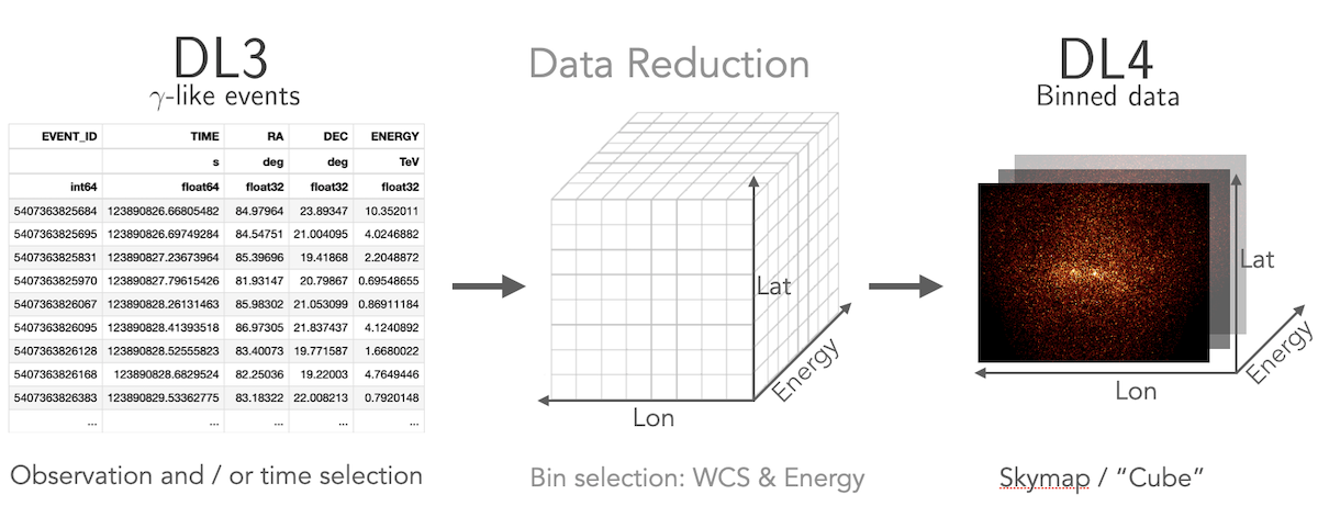
Gammapy lets you perform a combined spectral and spatial analysis as well.
This is sometimes called in jargon a “cube analysis”. Based on the 3D data reduction
Gammapy can also simulate events. Flux points can be computed using the
FluxPointsEstimator.
3D analysis tutorial 3D analysis tutorial with event sampling
Gammapy allows you to compute light curves in various ways. Light curves
can be computed for a 1D or 3D analysis scenario (see above) by either
grouping or splitting the DL3 data into multiple time intervals. Grouping
mutiple observations allows for computing e.g. a monthly or nightly light curves,
while splitting of a single observation allows to compute light curves for flares.
You can also compute light curves in multiple energy bands. In all cases the light
curve is computed using the LightCurveEstimator.
Gammapy offers the possibility to combine data from multiple instruments in a “joint-likelihood” fit. This can be done at multiple data levels and independent dimensionality of the data. Gammapy can handle 1D and 3D datasets at the same time and can also include e.g. flux points in a combined likelihood fit.