This is a fixed-text formatted version of a Jupyter notebook
Try online

You may download all the notebooks as a tar file.
Source files: analysis_3d.ipynb | analysis_3d.py
3D detailed analysis#
This tutorial does a 3D map based analsis on the galactic center, using simulated observations from the CTA-1DC. We will use the high level interface for the data reduction, and then do a detailed modelling. This will be done in two different ways:
stacking all the maps together and fitting the stacked maps
handling all the observations separately and doing a joint fitting on all the maps
[1]:
%matplotlib inline
import matplotlib.pyplot as plt
import numpy as np
import astropy.units as u
from pathlib import Path
from regions import CircleSkyRegion
from scipy.stats import norm
from gammapy.analysis import Analysis, AnalysisConfig
from gammapy.modeling.models import (
    SkyModel,
    ExpCutoffPowerLawSpectralModel,
    PointSpatialModel,
    FoVBackgroundModel,
    Models,
)
from gammapy.modeling import Fit
from gammapy.maps import Map
from gammapy.estimators import ExcessMapEstimator
from gammapy.datasets import MapDataset
Analysis configuration#
In this section we select observations and define the analysis geometries, irrespective of joint/stacked analysis. For configuration of the analysis, we will programmatically build a config file from scratch.
[2]:
config = AnalysisConfig()
# The config file is now empty, with only a few defaults specified.
print(config)
AnalysisConfig

    general:
        log: {level: info, filename: null, filemode: null, format: null, datefmt: null}
        outdir: .
        n_jobs: 1
        datasets_file: null
        models_file: null
    observations:
        datastore: $GAMMAPY_DATA/hess-dl3-dr1
        obs_ids: []
        obs_file: null
        obs_cone: {frame: null, lon: null, lat: null, radius: null}
        obs_time: {start: null, stop: null}
        required_irf: [aeff, edisp, psf, bkg]
    datasets:
        type: 1d
        stack: true
        geom:
            wcs:
                skydir: {frame: null, lon: null, lat: null}
                binsize: 0.02 deg
                width: {width: 5.0 deg, height: 5.0 deg}
                binsize_irf: 0.2 deg
            selection: {offset_max: 2.5 deg}
            axes:
                energy: {min: 1.0 TeV, max: 10.0 TeV, nbins: 5}
                energy_true: {min: 0.5 TeV, max: 20.0 TeV, nbins: 16}
        map_selection: [counts, exposure, background, psf, edisp]
        background:
            method: null
            exclusion: null
            parameters: {}
        safe_mask:
            methods: [aeff-default]
            parameters: {}
        on_region: {frame: null, lon: null, lat: null, radius: null}
        containment_correction: true
    fit:
        fit_range: {min: null, max: null}
    flux_points:
        energy: {min: null, max: null, nbins: null}
        source: source
        parameters: {selection_optional: all}
    excess_map:
        correlation_radius: 0.1 deg
        parameters: {}
        energy_edges: {min: null, max: null, nbins: null}
    light_curve:
        time_intervals: {start: null, stop: null}
        energy_edges: {min: null, max: null, nbins: null}
        source: source
        parameters: {selection_optional: all}
[3]:
# Selecting the observations
config.observations.datastore = "$GAMMAPY_DATA/cta-1dc/index/gps/"
config.observations.obs_ids = [110380, 111140, 111159]
[4]:
# Defining a reference geometry for the reduced datasets

config.datasets.type = "3d"  # Analysis type is 3D

config.datasets.geom.wcs.skydir = {
    "lon": "0 deg",
    "lat": "0 deg",
    "frame": "galactic",
}  # The WCS geometry - centered on the galactic center
config.datasets.geom.wcs.width = {"width": "10 deg", "height": "8 deg"}
config.datasets.geom.wcs.binsize = "0.02 deg"

# Cutout size (for the run-wise event selection)
config.datasets.geom.selection.offset_max = 3.5 * u.deg
config.datasets.safe_mask.methods = ["aeff-default", "offset-max"]

# We now fix the energy axis for the counts map - (the reconstructed energy binning)
config.datasets.geom.axes.energy.min = "0.1 TeV"
config.datasets.geom.axes.energy.max = "10 TeV"
config.datasets.geom.axes.energy.nbins = 10

# We now fix the energy axis for the IRF maps (exposure, etc) - (the true energy binning)
config.datasets.geom.axes.energy_true.min = "0.08 TeV"
config.datasets.geom.axes.energy_true.max = "12 TeV"
config.datasets.geom.axes.energy_true.nbins = 14
[5]:
print(config)
AnalysisConfig

    general:
        log: {level: info, filename: null, filemode: null, format: null, datefmt: null}
        outdir: .
        n_jobs: 1
        datasets_file: null
        models_file: null
    observations:
        datastore: $GAMMAPY_DATA/cta-1dc/index/gps
        obs_ids: [110380, 111140, 111159]
        obs_file: null
        obs_cone: {frame: null, lon: null, lat: null, radius: null}
        obs_time: {start: null, stop: null}
        required_irf: [aeff, edisp, psf, bkg]
    datasets:
        type: 3d
        stack: true
        geom:
            wcs:
                skydir: {frame: galactic, lon: 0.0 deg, lat: 0.0 deg}
                binsize: 0.02 deg
                width: {width: 10.0 deg, height: 8.0 deg}
                binsize_irf: 0.2 deg
            selection: {offset_max: 3.5 deg}
            axes:
                energy: {min: 0.1 TeV, max: 10.0 TeV, nbins: 10}
                energy_true: {min: 0.08 TeV, max: 12.0 TeV, nbins: 14}
        map_selection: [counts, exposure, background, psf, edisp]
        background:
            method: null
            exclusion: null
            parameters: {}
        safe_mask:
            methods: [aeff-default, offset-max]
            parameters: {}
        on_region: {frame: null, lon: null, lat: null, radius: null}
        containment_correction: true
    fit:
        fit_range: {min: null, max: null}
    flux_points:
        energy: {min: null, max: null, nbins: null}
        source: source
        parameters: {selection_optional: all}
    excess_map:
        correlation_radius: 0.1 deg
        parameters: {}
        energy_edges: {min: null, max: null, nbins: null}
    light_curve:
        time_intervals: {start: null, stop: null}
        energy_edges: {min: null, max: null, nbins: null}
        source: source
        parameters: {selection_optional: all}
Configuration for stacked and joint analysis#
This is done just by specfiying the flag on config.datasets.stack. Since the internal machinery will work differently for the two cases, we will write it as two config files and save it to disc in YAML format for future reference.
[6]:
config_stack = config.copy(deep=True)
config_stack.datasets.stack = True

config_joint = config.copy(deep=True)
config_joint.datasets.stack = False
[7]:
# To prevent unnecessary cluttering, we write it in a separate folder.
path = Path("analysis_3d")
path.mkdir(exist_ok=True)
config_joint.write(path=path / "config_joint.yaml", overwrite=True)
config_stack.write(path=path / "config_stack.yaml", overwrite=True)
Stacked analysis#
Data reduction#
We first show the steps for the stacked analysis and then repeat the same for the joint analysis later
[8]:
# Reading yaml file:
config_stacked = AnalysisConfig.read(path=path / "config_stack.yaml")
[9]:
analysis_stacked = Analysis(config_stacked)
Setting logging config: {'level': 'INFO', 'filename': None, 'filemode': None, 'format': None, 'datefmt': None}
[10]:
%%time
# select observations:
analysis_stacked.get_observations()

# run data reduction
analysis_stacked.get_datasets()
Fetching observations.
Observations selected: 3 out of 3.
Number of selected observations: 3
Creating reference dataset and makers.
Creating the background Maker.
No background maker set. Check configuration.
Start the data reduction loop.
Computing dataset for observation 110380
Running MapDatasetMaker
Invalid unit found in background table! Assuming (s-1 MeV-1 sr-1)
Running SafeMaskMaker
No default upper safe energy threshold defined for obs 110380
No default lower safe energy threshold defined for obs 110380
Computing dataset for observation 111140
Running MapDatasetMaker
Invalid unit found in background table! Assuming (s-1 MeV-1 sr-1)
Running SafeMaskMaker
No default upper safe energy threshold defined for obs 111140
No default lower safe energy threshold defined for obs 111140
Computing dataset for observation 111159
Running MapDatasetMaker
Invalid unit found in background table! Assuming (s-1 MeV-1 sr-1)
Running SafeMaskMaker
No default upper safe energy threshold defined for obs 111159
No default lower safe energy threshold defined for obs 111159
CPU times: user 9.62 s, sys: 1.97 s, total: 11.6 s
Wall time: 14.2 s
We have one final dataset, which you can print and explore
[11]:
dataset_stacked = analysis_stacked.datasets["stacked"]
print(dataset_stacked)
MapDataset
----------

  Name                            : stacked

  Total counts                    : 121241
  Total background counts         : 108043.52
  Total excess counts             : 13197.48

  Predicted counts                : 108043.52
  Predicted background counts     : 108043.52
  Predicted excess counts         : nan

  Exposure min                    : 6.28e+07 m2 s
  Exposure max                    : 1.90e+10 m2 s

  Number of total bins            : 2000000
  Number of fit bins              : 1411180

  Fit statistic type              : cash
  Fit statistic value (-2 log(L)) : nan

  Number of models                : 0
  Number of parameters            : 0
  Number of free parameters       : 0
[12]:
# To plot a smooth counts map
dataset_stacked.counts.smooth(0.02 * u.deg).plot_interactive(add_cbar=True)
[13]:
# And the background map
dataset_stacked.background.plot_interactive(add_cbar=True)
[14]:
# We can quickly check the PSF
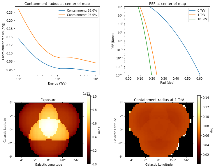
dataset_stacked.psf.peek()
[15]:
# And the energy dispersion in the center of the map
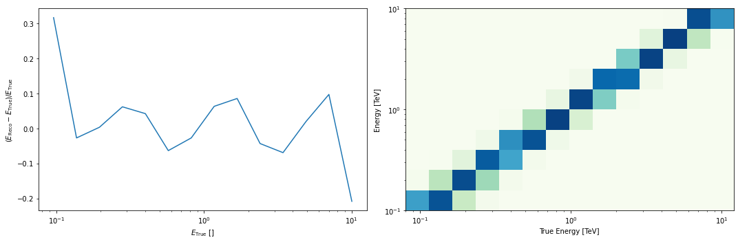
dataset_stacked.edisp.peek()
[16]:
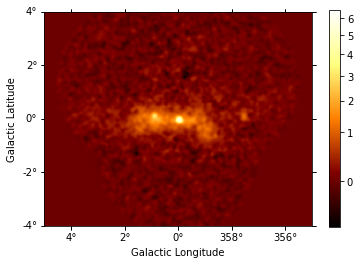
# You can also get an excess image with a few lines of code:
excess = dataset_stacked.excess.sum_over_axes()
excess.smooth("0.06 deg").plot(stretch="sqrt", add_cbar=True);
Modeling and fitting#
Now comes the interesting part of the analysis - choosing appropriate models for our source and fitting them.
We choose a point source model with an exponential cutoff power-law spectrum.
To perform the fit on a restricted energy range, we can create a specific mask. On the dataset, the mask_fit is a Map sharing the same geometry as the MapDataset and containing boolean data.
To create a mask to limit the fit within a restricted energy range, one can rely on the gammapy.maps.Geom.energy_mask() method.
For more details on masks and the techniques to create them in gammapy, please refer to the dedicated tutorial
[17]:
dataset_stacked.mask_fit = dataset_stacked.counts.geom.energy_mask(
    energy_min=0.3 * u.TeV, energy_max=None
)
[18]:
spatial_model = PointSpatialModel(
    lon_0="-0.05 deg", lat_0="-0.05 deg", frame="galactic"
)
spectral_model = ExpCutoffPowerLawSpectralModel(
    index=2.3,
    amplitude=2.8e-12 * u.Unit("cm-2 s-1 TeV-1"),
    reference=1.0 * u.TeV,
    lambda_=0.02 / u.TeV,
)

model = SkyModel(
    spatial_model=spatial_model,
    spectral_model=spectral_model,
    name="gc-source",
)

bkg_model = FoVBackgroundModel(dataset_name="stacked")
bkg_model.spectral_model.norm.value = 1.3

models_stacked = Models([model, bkg_model])

dataset_stacked.models = models_stacked
[19]:
%%time
fit = Fit(optimize_opts={"print_level": 1})
result = fit.run(datasets=[dataset_stacked])
CPU times: user 6.67 s, sys: 2 s, total: 8.67 s
Wall time: 11.4 s
Fit quality assessment and model residuals for a MapDataset#
We can access the results dictionary to see if the fit converged:
[20]:
print(result)
OptimizeResult

        backend    : minuit
        method     : migrad
        success    : True
        message    : Optimization terminated successfully.
        nfev       : 182
        total stat : 180458.06

CovarianceResult

        backend    : minuit
        method     : hesse
        success    : True
        message    : Hesse terminated successfully.
Check best-fit parameters and error estimates:
[21]:
models_stacked.to_parameters_table()
[21]:
| model | type | name | value | unit | error | min | max | frozen | is_norm | link |
|---|---|---|---|---|---|---|---|---|---|---|
| str11 | str8 | str9 | float64 | str14 | float64 | float64 | float64 | bool | bool | str1 |
| gc-source | spectral | index | 2.4147e+00 | 1.522e-01 | nan | nan | False | False | ||
| gc-source | spectral | amplitude | 2.6624e-12 | cm-2 s-1 TeV-1 | 3.103e-13 | nan | nan | False | True | |
| gc-source | spectral | reference | 1.0000e+00 | TeV | 0.000e+00 | nan | nan | True | False | |
| gc-source | spectral | lambda_ | -1.3517e-02 | TeV-1 | 6.837e-02 | nan | nan | False | False | |
| gc-source | spectral | alpha | 1.0000e+00 | 0.000e+00 | nan | nan | True | False | ||
| gc-source | spatial | lon_0 | -4.8065e-02 | deg | 2.286e-03 | nan | nan | False | False | |
| gc-source | spatial | lat_0 | -5.2605e-02 | deg | 2.262e-03 | -9.000e+01 | 9.000e+01 | False | False | |
| stacked-bkg | spectral | norm | 1.3481e+00 | 9.315e-03 | nan | nan | False | True | ||
| stacked-bkg | spectral | tilt | 0.0000e+00 | 0.000e+00 | nan | nan | True | False | ||
| stacked-bkg | spectral | reference | 1.0000e+00 | TeV | 0.000e+00 | nan | nan | True | False |
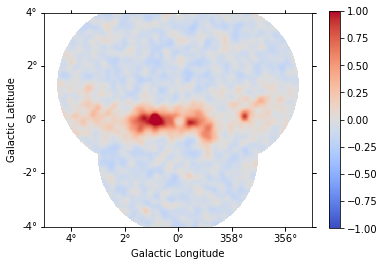
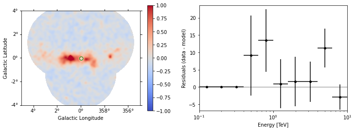
A quick way to inspect the model residuals is using the function ~MapDataset.plot_residuals_spatial(). This function computes and plots a residual image (by default, the smoothing radius is 0.1 deg and method=diff, which corresponds to a simple data - model plot):
[22]:
dataset_stacked.plot_residuals_spatial(
    method="diff/sqrt(model)", vmin=-1, vmax=1
);
The more general function ~MapDataset.plot_residuals() can also extract and display spectral residuals in a region:
[23]:
region = CircleSkyRegion(spatial_model.position, radius=0.15 * u.deg)

dataset_stacked.plot_residuals(
    kwargs_spatial=dict(method="diff/sqrt(model)", vmin=-1, vmax=1),
    kwargs_spectral=dict(region=region),
);
This way of accessing residuals is quick and handy, but comes with limitations. For example: - In case a fitting energy range was defined using a MapDataset.mask_fit, it won’t be taken into account. Residuals will be summed up over the whole reconstructed energy range - In order to make a proper statistic treatment, instead of simple residuals a proper residuals significance map should be computed
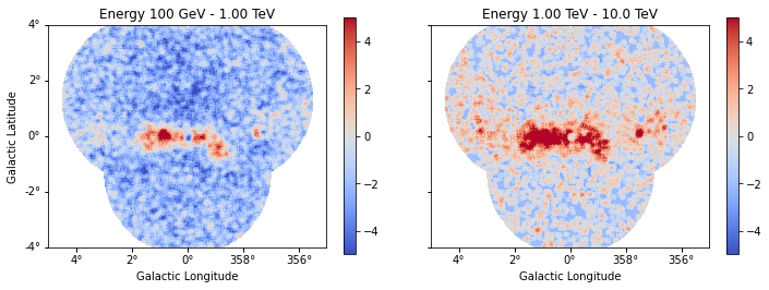
A more accurate way to inspect spatial residuals is the following:
[24]:
estimator = ExcessMapEstimator(
    correlation_radius="0.1 deg",
    selection_optional=[],
    energy_edges=[0.1, 1, 10] * u.TeV,
)

result = estimator.run(dataset_stacked)

result["sqrt_ts"].plot_grid(
    figsize=(12, 4), cmap="coolwarm", add_cbar=True, vmin=-5, vmax=5, ncols=2
);
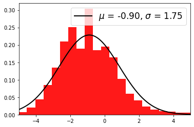
Distribution of residuals significance in the full map geometry:
[25]:
# TODO: clean this up
significance_data = result["sqrt_ts"].data

# #Remove bins that are inside an exclusion region, that would create an artificial peak at significance=0.
# #For now these lines are useless, because to_image() drops the mask fit
# mask_data = dataset_image.mask_fit.sum_over_axes().data
# excluded = mask_data == 0
# significance_data = significance_data[~excluded]
selection = np.isfinite(significance_data) & ~(significance_data == 0)
significance_data = significance_data[selection]

plt.hist(significance_data, density=True, alpha=0.9, color="red", bins=40)
mu, std = norm.fit(significance_data)

x = np.linspace(-5, 5, 100)
p = norm.pdf(x, mu, std)

plt.plot(
    x,
    p,
    lw=2,
    color="black",
    label=r"$\mu$ = {:.2f}, $\sigma$ = {:.2f}".format(mu, std),
)
plt.legend(fontsize=17)
plt.xlim(-5, 5)
[25]:
(-5.0, 5.0)
Joint analysis#
In this section, we perform a joint analysis of the same data. Of course, joint fitting is considerably heavier than stacked one, and should always be handled with care. For brevity, we only show the analysis for a point source fitting without re-adding a diffuse component again.
Data reduction#
[26]:
%%time

# Read the yaml file from disk
config_joint = AnalysisConfig.read(path=path / "config_joint.yaml")
analysis_joint = Analysis(config_joint)

# select observations:
analysis_joint.get_observations()

# run data reduction
analysis_joint.get_datasets()
Setting logging config: {'level': 'INFO', 'filename': None, 'filemode': None, 'format': None, 'datefmt': None}
Fetching observations.
Observations selected: 3 out of 3.
Number of selected observations: 3
Creating reference dataset and makers.
Creating the background Maker.
No background maker set. Check configuration.
Start the data reduction loop.
Computing dataset for observation 110380
Running MapDatasetMaker
Invalid unit found in background table! Assuming (s-1 MeV-1 sr-1)
Running SafeMaskMaker
No default upper safe energy threshold defined for obs 110380
No default lower safe energy threshold defined for obs 110380
Computing dataset for observation 111140
Running MapDatasetMaker
Invalid unit found in background table! Assuming (s-1 MeV-1 sr-1)
Running SafeMaskMaker
No default upper safe energy threshold defined for obs 111140
No default lower safe energy threshold defined for obs 111140
Computing dataset for observation 111159
Running MapDatasetMaker
Invalid unit found in background table! Assuming (s-1 MeV-1 sr-1)
Running SafeMaskMaker
No default upper safe energy threshold defined for obs 111159
No default lower safe energy threshold defined for obs 111159
CPU times: user 9.35 s, sys: 1.78 s, total: 11.1 s
Wall time: 13.7 s
[27]:
# You can see there are 3 datasets now
print(analysis_joint.datasets)
Datasets
--------

Dataset 0:

  Type       : MapDataset
  Name       : elj9nx1B
  Instrument : CTA
  Models     :

Dataset 1:

  Type       : MapDataset
  Name       : QTQBDWWL
  Instrument : CTA
  Models     :

Dataset 2:

  Type       : MapDataset
  Name       : 339EAxR_
  Instrument : CTA
  Models     :
[28]:
# You can access each one by name or by index, eg:
print(analysis_joint.datasets[0])
MapDataset
----------

  Name                            : elj9nx1B

  Total counts                    : 40481
  Total background counts         : 36014.51
  Total excess counts             : 4466.49

  Predicted counts                : 36014.51
  Predicted background counts     : 36014.51
  Predicted excess counts         : nan

  Exposure min                    : 6.28e+07 m2 s
  Exposure max                    : 6.68e+09 m2 s

  Number of total bins            : 1085000
  Number of fit bins              : 693940

  Fit statistic type              : cash
  Fit statistic value (-2 log(L)) : nan

  Number of models                : 0
  Number of parameters            : 0
  Number of free parameters       : 0
After the data reduction stage, it is nice to get a quick summary info on the datasets. Here, we look at the statistics in the center of Map, by passing an appropriate region. To get info on the entire spatial map, omit the region argument.
[29]:
analysis_joint.datasets.info_table()
[29]:
| name | counts | excess | sqrt_ts | background | npred | npred_background | npred_signal | exposure_min | exposure_max | livetime | ontime | counts_rate | background_rate | excess_rate | n_bins | n_fit_bins | stat_type | stat_sum |
|---|---|---|---|---|---|---|---|---|---|---|---|---|---|---|---|---|---|---|
| m2 s | m2 s | s | s | 1 / s | 1 / s | 1 / s | ||||||||||||
| str8 | int64 | float64 | float64 | float64 | float64 | float64 | float64 | float64 | float64 | float64 | float64 | float64 | float64 | float64 | int64 | int64 | str4 | float64 |
| elj9nx1B | 40481 | 4466.484375 | 23.07275543163338 | 36014.515625 | 36014.50702797074 | 36014.515625 | nan | 62838924.0 | 6676807680.0 | 1764.000034326 | 1800.0 | 22.948412251855327 | 20.416391680378084 | 2.5320205714772457 | 1085000 | 693940 | cash | nan |
| QTQBDWWL | 40525 | 4510.505455516504 | 23.29577792435477 | 36014.494544483496 | 36014.494544483496 | 36014.494544483496 | nan | 62838194.40984807 | 6676808531.804668 | 1764.000034326 | 1800.0 | 22.97335556202755 | 20.41637972997213 | 2.556975832055415 | 1085000 | 693940 | cash | nan |
| 339EAxR_ | 40235 | 4220.48048722629 | 21.824963885829067 | 36014.51951277371 | 36014.51951277371 | 36014.51951277371 | nan | 62838404.53574324 | 6676813626.917053 | 1764.000034326 | 1800.0 | 22.8089564722561 | 20.416393884331388 | 2.3925625879247088 | 1085000 | 693940 | cash | nan |
[30]:
models_joint = Models()

model_joint = model.copy(name="source-joint")
models_joint.append(model_joint)

for dataset in analysis_joint.datasets:
    bkg_model = FoVBackgroundModel(dataset_name=dataset.name)
    models_joint.append(bkg_model)

print(models_joint)
Models

Component 0: SkyModel

  Name                      : source-joint
  Datasets names            : None
  Spectral model type       : ExpCutoffPowerLawSpectralModel
  Spatial  model type       : PointSpatialModel
  Temporal model type       :
  Parameters:
    index                         :      2.415   +/-    0.15
    amplitude                     :   2.66e-12   +/- 3.1e-13 1 / (cm2 s TeV)
    reference             (frozen):      1.000       TeV
    lambda_                       :     -0.014   +/-    0.07 1 / TeV
    alpha                 (frozen):      1.000
    lon_0                         :     -0.048   +/-    0.00 deg
    lat_0                         :     -0.053   +/-    0.00 deg

Component 1: FoVBackgroundModel

  Name                      : elj9nx1B-bkg
  Datasets names            : ['elj9nx1B']
  Spectral model type       : PowerLawNormSpectralModel
  Parameters:
    norm                          :      1.000   +/-    0.00
    tilt                  (frozen):      0.000
    reference             (frozen):      1.000       TeV

Component 2: FoVBackgroundModel

  Name                      : QTQBDWWL-bkg
  Datasets names            : ['QTQBDWWL']
  Spectral model type       : PowerLawNormSpectralModel
  Parameters:
    norm                          :      1.000   +/-    0.00
    tilt                  (frozen):      0.000
    reference             (frozen):      1.000       TeV

Component 3: FoVBackgroundModel

  Name                      : 339EAxR_-bkg
  Datasets names            : ['339EAxR_']
  Spectral model type       : PowerLawNormSpectralModel
  Parameters:
    norm                          :      1.000   +/-    0.00
    tilt                  (frozen):      0.000
    reference             (frozen):      1.000       TeV
[31]:
# and set the new model
analysis_joint.datasets.models = models_joint
[32]:
%%time
fit_joint = Fit()
result_joint = fit_joint.run(datasets=analysis_joint.datasets)
CPU times: user 10.9 s, sys: 2.1 s, total: 13 s
Wall time: 15 s
Fit quality assessment and model residuals for a joint Datasets#
We can access the results dictionary to see if the fit converged:
[33]:
print(result_joint)
OptimizeResult

        backend    : minuit
        method     : migrad
        success    : True
        message    : Optimization terminated successfully.
        nfev       : 238
        total stat : 748259.16

CovarianceResult

        backend    : minuit
        method     : hesse
        success    : True
        message    : Hesse terminated successfully.
Check best-fit parameters and error estimates:
[34]:
print(models_joint)
Models

Component 0: SkyModel

  Name                      : source-joint
  Datasets names            : None
  Spectral model type       : ExpCutoffPowerLawSpectralModel
  Spatial  model type       : PointSpatialModel
  Temporal model type       :
  Parameters:
    index                         :      2.272   +/-    0.08
    amplitude                     :   2.84e-12   +/- 3.1e-13 1 / (cm2 s TeV)
    reference             (frozen):      1.000       TeV
    lambda_                       :      0.039   +/-    0.05 1 / TeV
    alpha                 (frozen):      1.000
    lon_0                         :     -0.049   +/-    0.00 deg
    lat_0                         :     -0.053   +/-    0.00 deg

Component 1: FoVBackgroundModel

  Name                      : elj9nx1B-bkg
  Datasets names            : ['elj9nx1B']
  Spectral model type       : PowerLawNormSpectralModel
  Parameters:
    norm                          :      1.118   +/-    0.01
    tilt                  (frozen):      0.000
    reference             (frozen):      1.000       TeV

Component 2: FoVBackgroundModel

  Name                      : QTQBDWWL-bkg
  Datasets names            : ['QTQBDWWL']
  Spectral model type       : PowerLawNormSpectralModel
  Parameters:
    norm                          :      1.119   +/-    0.01
    tilt                  (frozen):      0.000
    reference             (frozen):      1.000       TeV

Component 3: FoVBackgroundModel

  Name                      : 339EAxR_-bkg
  Datasets names            : ['339EAxR_']
  Spectral model type       : PowerLawNormSpectralModel
  Parameters:
    norm                          :      1.111   +/-    0.01
    tilt                  (frozen):      0.000
    reference             (frozen):      1.000       TeV
Since the joint dataset is made of multiple datasets, we can either: - Look at the residuals for each dataset separately. In this case, we can directly refer to the section Fit quality and model residuals for a MapDataset in this notebook - Look at a stacked residual map.
In the latter case, we need to properly stack the joint dataset before computing the residuals:
[35]:
# TODO: clean this up

# We need to stack on the full geometry, so we use to geom from the stacked counts map.
stacked = MapDataset.from_geoms(**dataset_stacked.geoms)

for dataset in analysis_joint.datasets:
    # TODO: Apply mask_fit before stacking
    stacked.stack(dataset)

stacked.models = [model_joint]
[36]:
stacked.plot_residuals_spatial(vmin=-1, vmax=1);
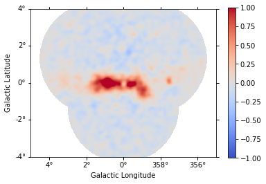
Then, we can access the stacked model residuals as previously shown in the section Fit quality and model residuals for a MapDataset in this notebook.
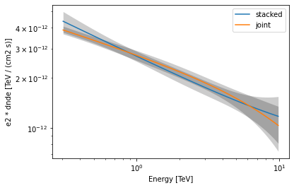
Finally, let us compare the spectral results from the stacked and joint fit:
[37]:
def plot_spectrum(model, result, label, color):
    spec = model.spectral_model
    energy_bounds = [0.3, 10] * u.TeV
    spec.plot(
        energy_bounds=energy_bounds, energy_power=2, label=label, color=color
    )
    spec.plot_error(energy_bounds=energy_bounds, energy_power=2, color=color)
[38]:
plot_spectrum(model, result, label="stacked", color="tab:blue")
plot_spectrum(model_joint, result_joint, label="joint", color="tab:orange")
plt.legend()
[38]:
<matplotlib.legend.Legend at 0x1761169a0>
Summary#
Note that this notebook aims to show you the procedure of a 3D analysis using just a few observations. Results get much better for a more complete analysis considering the GPS dataset from the CTA First Data Challenge (DC-1) and also the CTA model for the Galactic diffuse emission, as shown in the next image:
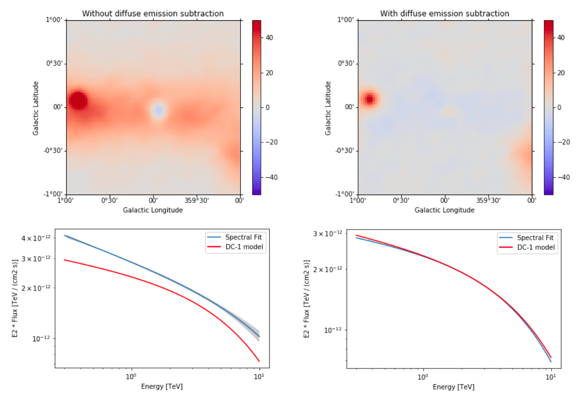
The complete tutorial notebook of this analysis is available to be downloaded in GAMMAPY-EXTRA repository at https://github.com/gammapy/gammapy-extra/blob/master/analyses/cta_1dc_gc_3d.ipynb).
Exercises#
Analyse the second source in the field of view: G0.9+0.1 and add it to the combined model.
Perform modeling in more details - Add diffuse component, get flux points.