This is a fixed-text formatted version of a Jupyter notebook
Try online

You may download all the notebooks as a tar file.
Source files: flux_profiles.ipynb | flux_profiles.py
Flux Profile Estimation#
This tutorial shows how to estimate flux profiles.
Prerequisites#
Knowledge of 3D data reduction and datasets used in Gammapy, see for instance the first analysis tutorial.
Context#
A useful tool to study and compare the saptial distribution of flux in images and data cubes is the measurement of flxu profiles. Flux profiles can show spatial correlations of gamma-ray data with e.g. gas maps or other type of gamma-ray data. Most commonly flux profiles are measured along some preferred coordinate axis, either radially distance from a source of interest, along longitude and latitude coordinate axes or along the path defined by two spatial coordinates.
Proposed Approach#
Flux profile estimation essentially works by estimating flux points for a set of predefined spatially connected regions. For radial flux profiles the shape of the regions are annuli with a common center, for linear profiles it’s typically a rectangular shape.
We will work on a pre-computed MapDataset of Fermi-LAT data, use Region to define the structure of the bins of the flux profile and run the actually profile extraction using the FluxProfileEstimator
Setup and Imports#
[1]:
%matplotlib inline
import matplotlib.pyplot as plt
from astropy import units as u
from astropy.coordinates import SkyCoord
import numpy as np
[2]:
from gammapy.datasets import MapDataset
from gammapy.estimators import FluxProfileEstimator, FluxPoints
from gammapy.maps import RegionGeom
from gammapy.utils.regions import (
    make_concentric_annulus_sky_regions,
    make_orthogonal_rectangle_sky_regions,
)
from gammapy.modeling.models import PowerLawSpectralModel
Read and Introduce Data#
[3]:
dataset = MapDataset.read(
    "$GAMMAPY_DATA/fermi-3fhl-gc/fermi-3fhl-gc.fits.gz", name="fermi-dataset"
)
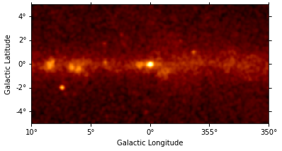
This is what the counts image we will work with looks like:
[4]:
counts_image = dataset.counts.sum_over_axes()
counts_image.smooth("0.1 deg").plot(stretch="sqrt");
There are 400x200 pixels in the dataset and 11 energy bins between 10 GeV and 2 TeV:
[5]:
print(dataset.counts)
WcsNDMap

        geom  : WcsGeom
        axes  : ['lon', 'lat', 'energy']
        shape : (400, 200, 11)
        ndim  : 3
        unit  :
        dtype : >i4
Profile Estimation#
Configuration#
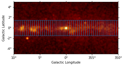
We start by defining a list of spatially connected regions along the galactic longitude axis. For this there is a helper function make_orthogonal_rectangle_sky_regions. The individual region bins for the profile have a height of 3 deg and in total there are 31 bins. The starts from lon = 10 deg tand goes to lon = 350 deg. In addition we have to specify the wcs to take into account possible projections effects on the region definition:
[6]:
regions = make_orthogonal_rectangle_sky_regions(
    start_pos=SkyCoord("10d", "0d", frame="galactic"),
    end_pos=SkyCoord("350d", "0d", frame="galactic"),
    wcs=counts_image.geom.wcs,
    height="3 deg",
    nbin=51,
)
We can use the RegionGeom object to illustrate the regions on top of the counts image:
[7]:
geom = RegionGeom.create(region=regions)
ax = counts_image.smooth("0.1 deg").plot(stretch="sqrt")
geom.plot_region(ax=ax, color="w");
/Users/adonath/software/mambaforge/envs/gammapy-dev/lib/python3.9/site-packages/regions/shapes/rectangle.py:201: UserWarning: Setting the 'color' property will override the edgecolor or facecolor properties.
  return Rectangle(xy=xy, width=width, height=height,
Next we create the FluxProfileEstimator. For the estimation of the flux profile we assume a spectral model with a power-law shape and an index of 2.3
[8]:
flux_profile_estimator = FluxProfileEstimator(
    regions=regions,
    spectrum=PowerLawSpectralModel(index=2.3),
    energy_edges=[10, 2000] * u.GeV,
    selection_optional=["ul"],
)
We can see the full configuration by printing the estimator object:
[9]:
print(flux_profile_estimator)
FluxProfileEstimator
--------------------

  energy_edges           : [  10. 2000.] GeV
  fit                    : <gammapy.modeling.fit.Fit object at 0x174b100d0>
  n_sigma                : 1
  n_sigma_ul             : 2
  norm_max               : 5
  norm_min               : 0.2
  norm_n_values          : 11
  norm_values            : None
  null_value             : 0
  reoptimize             : False
  selection_optional     : ['ul']
  source                 : 0
  spectrum               : PowerLawSpectralModel
  sum_over_energy_groups : False
Run Estimation#
Now we can run the profile estimation and explore the results:
[10]:
%%time
profile = flux_profile_estimator.run(datasets=dataset)
CPU times: user 16.8 s, sys: 391 ms, total: 17.2 s
Wall time: 22 s
[11]:
print(profile)
FluxPoints
----------

  geom                   : RegionGeom
  axes                   : ['lon', 'lat', 'energy', 'projected-distance']
  shape                  : (1, 1, 1, 51)
  quantities             : ['norm', 'norm_err', 'norm_ul', 'ts', 'npred', 'npred_excess', 'stat', 'counts', 'success']
  ref. model             : pl
  n_sigma                : 1
  n_sigma_ul             : 2
  sqrt_ts_threshold_ul   : 2
  sed type init          : likelihood
We can see the flux profile is represented by a FluxPoints object with a projected-distance axis, which defines the main axis the flux profile is measured along. The lon and lat axes can be ignored.
Plotting Results#
Let us directly plot the result using FluxPoints.plot():
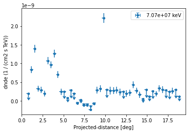
[12]:
ax = profile.plot(sed_type="dnde")
ax.set_yscale("linear")

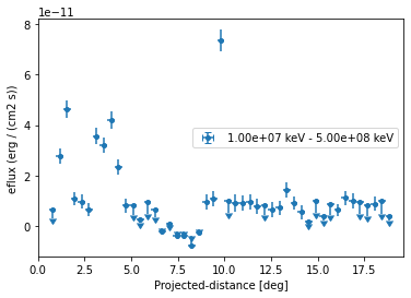
Based on the spectral model we specified above we can also plot in any other sed type, e.g. energy flux and define a different threshold when to plot upper limits:
[13]:
profile.sqrt_ts_threshold_ul = 2

ax = profile.plot(sed_type="eflux")
ax.set_yscale("linear")
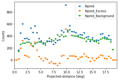
We can also plot any other quantity of interest, that is defined on the FluxPoints result object. E.g. the predicted total counts, background counts and excess counts:
[14]:
quantities = ["npred", "npred_excess", "npred_background"]

for quantity in quantities:
    profile[quantity].plot(label=quantity.title())

plt.ylabel("Counts ")
[14]:
Text(0, 0.5, 'Counts ')
Serialisation and I/O#
The profile can be serialised using FluxPoints.write(), given a specific format:
[15]:
profile.write(
    filename="flux_profile_fermi.fits",
    format="profile",
    overwrite=True,
    sed_type="dnde",
)
[16]:
profile_new = FluxPoints.read(
    filename="flux_profile_fermi.fits", format="profile"
)
No reference model set for FluxMaps. Assuming point source with E^-2 spectrum.
[17]:
ax = profile_new.plot()
ax.set_yscale("linear")
The profile can be serialised to a ~astropy.table.Table object using:
[18]:
table = profile.to_table(format="profile", formatted=True)
table
[18]:
| x_min | x_max | x_ref | e_ref [1] | e_min [1] | e_max [1] | ref_dnde [1] | ref_flux [1] | ref_eflux [1] | norm [1] | norm_err [1] | norm_ul [1] | ts [1] | sqrt_ts [1] | npred [1,1] | npred_excess [1,1] | stat [1] | is_ul [1] | counts [1,1] | success [1] |
|---|---|---|---|---|---|---|---|---|---|---|---|---|---|---|---|---|---|---|---|
| deg | deg | deg | keV | keV | keV | 1 / (cm2 s TeV) | keV / (cm2 s TeV) | keV2 / (cm2 s TeV) | |||||||||||
| float64 | float64 | float64 | float64 | float64 | float64 | float64 | float64 | float64 | float64 | float64 | float64 | float64 | float64 | float64 | float32 | float64 | bool | float64 | bool |
| -0.1960784313725492 | 0.1960784313725492 | 0.0 | 70710678.119 | 10000000.000 | 500000000.000 | 4.428e-10 | 3.043e-01 | 9.166e+06 | nan | nan | nan | nan | nan | nan | 0.0 | 0.000 | False | 0.0 | False |
| 0.1960784313725492 | 0.5882352941176467 | 0.392156862745098 | 70710678.119 | 10000000.000 | 500000000.000 | 4.428e-10 | 3.043e-01 | 9.166e+06 | nan | nan | nan | nan | nan | nan | 0.0 | 0.000 | False | 0.0 | False |
| 0.5882352941176467 | 0.9803921568627443 | 0.7843137254901955 | 70710678.119 | 10000000.000 | 500000000.000 | 4.428e-10 | 3.043e-01 | 9.166e+06 | 0.172 | 0.124 | 0.434 | 2.059 | 1.435 | 162.23048986115955 | 17.448376 | -818.848 | True | 163.0 | True |
| 0.9803921568627443 | 1.3725490196078436 | 1.176470588235294 | 70710678.119 | 10000000.000 | 500000000.000 | 4.428e-10 | 3.043e-01 | 9.166e+06 | 1.894 | 0.207 | 2.322 | 120.591 | 10.981 | 450.20181889217974 | 192.60909 | -3013.446 | False | 448.0 | True |
| 1.3725490196078436 | 1.764705882352942 | 1.5686274509803928 | 70710678.119 | 10000000.000 | 500000000.000 | 4.428e-10 | 3.043e-01 | 9.166e+06 | 3.146 | 0.240 | 3.639 | 280.648 | 16.753 | 601.6822045016994 | 320.15994 | -4348.966 | False | 599.0 | True |
| 1.764705882352942 | 2.15686274509804 | 1.960784313725491 | 70710678.119 | 10000000.000 | 500000000.000 | 4.428e-10 | 3.043e-01 | 9.166e+06 | 0.736 | 0.183 | 1.116 | 18.991 | 4.358 | 357.6650304886396 | 74.95968 | -2218.623 | False | 354.0 | True |
| 2.15686274509804 | 2.549019607843138 | 2.3529411764705888 | 70710678.119 | 10000000.000 | 500000000.000 | 4.428e-10 | 3.043e-01 | 9.166e+06 | 0.656 | 0.186 | 1.042 | 14.214 | 3.770 | 363.83338136609376 | 66.89659 | -2452.717 | False | 367.0 | True |
| 2.549019607843138 | 2.941176470588236 | 2.745098039215687 | 70710678.119 | 10000000.000 | 500000000.000 | 4.428e-10 | 3.043e-01 | 9.166e+06 | 0.450 | 0.179 | 0.821 | 7.011 | 2.648 | 339.4818273314676 | 45.943058 | -2174.005 | False | 339.0 | True |
| 2.941176470588236 | 3.3333333333333344 | 3.137254901960785 | 70710678.119 | 10000000.000 | 500000000.000 | 4.428e-10 | 3.043e-01 | 9.166e+06 | 2.421 | 0.225 | 2.885 | 174.146 | 13.196 | 528.0599574489612 | 247.276 | -3887.531 | False | 531.0 | True |
| 3.3333333333333344 | 3.725490196078432 | 3.529411764705883 | 70710678.119 | 10000000.000 | 500000000.000 | 4.428e-10 | 3.043e-01 | 9.166e+06 | 2.190 | 0.209 | 2.621 | 169.698 | 13.027 | 457.3561643542095 | 223.84384 | -3183.973 | False | 458.0 | True |
| 3.725490196078432 | 4.117647058823529 | 3.9215686274509807 | 70710678.119 | 10000000.000 | 500000000.000 | 4.428e-10 | 3.043e-01 | 9.166e+06 | 2.868 | 0.232 | 3.345 | 243.821 | 15.615 | 564.4775740614491 | 293.2505 | -4201.048 | False | 566.0 | True |
| 4.117647058823529 | 4.509803921568627 | 4.313725490196078 | 70710678.119 | 10000000.000 | 500000000.000 | 4.428e-10 | 3.043e-01 | 9.166e+06 | 1.599 | 0.205 | 2.023 | 81.901 | 9.050 | 451.76273200537855 | 163.63295 | -3040.782 | False | 448.0 | True |
| 4.509803921568627 | 4.901960784313727 | 4.7058823529411775 | 70710678.119 | 10000000.000 | 500000000.000 | 4.428e-10 | 3.043e-01 | 9.166e+06 | 0.550 | 0.182 | 0.928 | 10.243 | 3.201 | 356.28517250965956 | 56.336945 | -2313.852 | False | 356.0 | True |
| 4.901960784313727 | 5.294117647058824 | 5.098039215686276 | 70710678.119 | 10000000.000 | 500000000.000 | 4.428e-10 | 3.043e-01 | 9.166e+06 | 0.210 | 0.171 | 0.566 | 1.586 | 1.259 | 315.49805616415784 | 21.543198 | -1979.035 | True | 315.0 | True |
| 5.294117647058824 | 5.686274509803923 | 5.4901960784313735 | 70710678.119 | 10000000.000 | 500000000.000 | 4.428e-10 | 3.043e-01 | 9.166e+06 | -0.147 | 0.159 | 0.184 | 0.824 | -0.908 | 271.28752712430287 | -15.065349 | -1643.463 | True | 272.0 | True |
| 5.686274509803923 | 6.07843137254902 | 5.882352941176471 | 70710678.119 | 10000000.000 | 500000000.000 | 4.428e-10 | 3.043e-01 | 9.166e+06 | 0.302 | 0.162 | 0.640 | 3.766 | 1.941 | 282.32873883100837 | 31.023876 | -1692.050 | True | 282.0 | True |
| 6.07843137254902 | 6.470588235294118 | 6.274509803921569 | 70710678.119 | 10000000.000 | 500000000.000 | 4.428e-10 | 3.043e-01 | 9.166e+06 | 0.093 | 0.172 | 0.451 | 0.301 | 0.549 | 317.7330763355026 | 9.594112 | -2034.334 | True | 319.0 | True |
| 6.470588235294118 | 6.862745098039216 | 6.666666666666667 | 70710678.119 | 10000000.000 | 500000000.000 | 4.428e-10 | 3.043e-01 | 9.166e+06 | -0.500 | 0.170 | -0.147 | 7.804 | -2.794 | 311.3167047326352 | -51.37142 | -1931.193 | True | 311.0 | True |
| 6.862745098039216 | 7.254901960784315 | 7.058823529411765 | 70710678.119 | 10000000.000 | 500000000.000 | 4.428e-10 | 3.043e-01 | 9.166e+06 | -0.290 | 0.167 | 0.058 | 2.810 | -1.676 | 306.53518822433864 | -29.780603 | -1861.277 | True | 303.0 | True |
| 7.254901960784315 | 7.647058823529413 | 7.450980392156864 | 70710678.119 | 10000000.000 | 500000000.000 | 4.428e-10 | 3.043e-01 | 9.166e+06 | -0.590 | 0.155 | -0.267 | 12.500 | -3.536 | 261.73608142160793 | -60.75847 | -1577.587 | True | 263.0 | True |
| 7.647058823529413 | 8.039215686274511 | 7.843137254901962 | 70710678.119 | 10000000.000 | 500000000.000 | 4.428e-10 | 3.043e-01 | 9.166e+06 | -0.610 | 0.162 | -0.272 | 12.276 | -3.504 | 288.629200196315 | -62.79978 | -1754.528 | True | 288.0 | True |
| 8.039215686274511 | 8.43137254901961 | 8.235294117647062 | 70710678.119 | 10000000.000 | 500000000.000 | 4.428e-10 | 3.043e-01 | 9.166e+06 | -0.888 | 0.174 | -0.528 | 22.020 | -4.693 | 326.54526901543574 | -91.55885 | -2098.681 | True | 328.0 | True |
| ... | ... | ... | ... | ... | ... | ... | ... | ... | ... | ... | ... | ... | ... | ... | ... | ... | ... | ... | ... |
| 10.784313725490232 | 11.17647058823531 | 10.98039215686277 | 70710678.119 | 10000000.000 | 500000000.000 | 4.428e-10 | 3.043e-01 | 9.166e+06 | 0.629 | 0.209 | 1.061 | 9.978 | 3.159 | 474.3631284228803 | 65.154724 | -3224.239 | False | 473.0 | True |
| 11.17647058823531 | 11.568627450980387 | 11.372549019607849 | 70710678.119 | 10000000.000 | 500000000.000 | 4.428e-10 | 3.043e-01 | 9.166e+06 | 0.651 | 0.209 | 1.082 | 10.813 | 3.288 | 470.40241185983234 | 67.5138 | -3256.816 | False | 471.0 | True |
| 11.568627450980387 | 11.960784313725515 | 11.764705882352951 | 70710678.119 | 10000000.000 | 500000000.000 | 4.428e-10 | 3.043e-01 | 9.166e+06 | 0.517 | 0.204 | 0.939 | 6.975 | 2.641 | 451.98913792299624 | 53.64452 | -3129.927 | False | 453.0 | True |
| 11.960784313725515 | 12.352941176470619 | 12.156862745098067 | 70710678.119 | 10000000.000 | 500000000.000 | 4.428e-10 | 3.043e-01 | 9.166e+06 | 0.167 | 0.194 | 0.568 | 0.769 | 0.877 | 405.5267897789614 | 17.36149 | -2782.182 | True | 408.0 | True |
| 12.352941176470619 | 12.745098039215696 | 12.549019607843157 | 70710678.119 | 10000000.000 | 500000000.000 | 4.428e-10 | 3.043e-01 | 9.166e+06 | 0.441 | 0.197 | 0.848 | 5.381 | 2.320 | 424.9721062687647 | 45.757168 | -2877.351 | False | 425.0 | True |
| 12.745098039215696 | 13.137254901960773 | 12.941176470588236 | 70710678.119 | 10000000.000 | 500000000.000 | 4.428e-10 | 3.043e-01 | 9.166e+06 | 0.492 | 0.194 | 0.893 | 7.018 | 2.649 | 416.7588470906105 | 51.088707 | -2705.136 | False | 412.0 | True |
| 13.137254901960773 | 13.529411764705875 | 13.333333333333325 | 70710678.119 | 10000000.000 | 500000000.000 | 4.428e-10 | 3.043e-01 | 9.166e+06 | 0.959 | 0.205 | 1.382 | 25.879 | 5.087 | 455.22507305193835 | 99.72924 | -3216.032 | False | 458.0 | True |
| 13.529411764705875 | 13.921568627451002 | 13.72549019607844 | 70710678.119 | 10000000.000 | 500000000.000 | 4.428e-10 | 3.043e-01 | 9.166e+06 | 0.611 | 0.184 | 0.993 | 12.465 | 3.531 | 376.66733293729885 | 63.567978 | -2403.516 | False | 373.0 | True |
| 13.921568627451002 | 14.31372549019608 | 14.117647058823541 | 70710678.119 | 10000000.000 | 500000000.000 | 4.428e-10 | 3.043e-01 | 9.166e+06 | 0.377 | 0.187 | 0.763 | 4.407 | 2.099 | 385.1566764851361 | 39.272778 | -2526.278 | False | 384.0 | True |
| 14.31372549019608 | 14.705882352941185 | 14.509803921568633 | 70710678.119 | 10000000.000 | 500000000.000 | 4.428e-10 | 3.043e-01 | 9.166e+06 | -0.244 | 0.168 | 0.103 | 2.022 | -1.422 | 313.3736443463295 | -25.44988 | -1936.261 | True | 313.0 | True |
| 14.705882352941185 | 15.098039215686311 | 14.901960784313747 | 70710678.119 | 10000000.000 | 500000000.000 | 4.428e-10 | 3.043e-01 | 9.166e+06 | 0.307 | 0.179 | 0.679 | 3.133 | 1.770 | 366.322547445814 | 32.01158 | -2178.012 | True | 357.0 | True |
| 15.098039215686311 | 15.490196078431389 | 15.294117647058851 | 70710678.119 | 10000000.000 | 500000000.000 | 4.428e-10 | 3.043e-01 | 9.166e+06 | -0.083 | 0.167 | 0.265 | 0.240 | -0.490 | 313.4101919680869 | -8.618814 | -1914.901 | True | 311.0 | True |
| 15.490196078431389 | 15.882352941176466 | 15.686274509803926 | 70710678.119 | 10000000.000 | 500000000.000 | 4.428e-10 | 3.043e-01 | 9.166e+06 | 0.228 | 0.172 | 0.584 | 1.863 | 1.365 | 330.89113194006126 | 23.80037 | -2016.119 | True | 327.0 | True |
| 15.882352941176466 | 16.274509803921596 | 16.07843137254903 | 70710678.119 | 10000000.000 | 500000000.000 | 4.428e-10 | 3.043e-01 | 9.166e+06 | 0.427 | 0.170 | 0.780 | 6.979 | 2.642 | 324.69019708074285 | 44.554733 | -1957.576 | False | 321.0 | True |
| 16.274509803921596 | 16.666666666666696 | 16.470588235294144 | 70710678.119 | 10000000.000 | 500000000.000 | 4.428e-10 | 3.043e-01 | 9.166e+06 | 0.760 | 0.195 | 1.163 | 17.553 | 4.190 | 428.005206597181 | 79.45124 | -2767.621 | False | 421.0 | True |
| 16.666666666666696 | 17.058823529411775 | 16.862745098039234 | 70710678.119 | 10000000.000 | 500000000.000 | 4.428e-10 | 3.043e-01 | 9.166e+06 | 0.675 | 0.197 | 1.082 | 13.277 | 3.644 | 437.13415063137586 | 70.588745 | -2830.574 | False | 431.0 | True |
| 17.058823529411775 | 17.4509803921569 | 17.254901960784338 | 70710678.119 | 10000000.000 | 500000000.000 | 4.428e-10 | 3.043e-01 | 9.166e+06 | 0.256 | 0.183 | 0.634 | 2.057 | 1.434 | 381.24750962187824 | 26.727816 | -2356.744 | True | 374.0 | True |
| 17.4509803921569 | 17.843137254902004 | 17.647058823529452 | 70710678.119 | 10000000.000 | 500000000.000 | 4.428e-10 | 3.043e-01 | 9.166e+06 | 0.174 | 0.182 | 0.551 | 0.951 | 0.975 | 366.45334911783 | 18.242867 | -2463.364 | True | 370.0 | True |
| 17.843137254902004 | 18.235294117647083 | 18.039215686274545 | 70710678.119 | 10000000.000 | 500000000.000 | 4.428e-10 | 3.043e-01 | 9.166e+06 | 0.593 | 0.192 | 0.990 | 10.705 | 3.272 | 408.05504964497743 | 62.12828 | -2803.387 | False | 410.0 | True |
| 18.235294117647083 | 18.627450980392158 | 18.43137254901962 | 70710678.119 | 10000000.000 | 500000000.000 | 4.428e-10 | 3.043e-01 | 9.166e+06 | 0.306 | 0.173 | 0.666 | 3.342 | 1.828 | 334.14141424669504 | 32.074398 | -2186.572 | True | 336.0 | True |
| 18.627450980392158 | 19.01960784313726 | 18.82352941176471 | 70710678.119 | 10000000.000 | 500000000.000 | 4.428e-10 | 3.043e-01 | 9.166e+06 | 0.010 | 0.124 | 0.269 | 0.005 | 0.071 | 171.8115649139593 | 0.9959075 | -877.032 | True | 172.0 | True |
| 19.01960784313726 | 19.41176470588239 | 19.215686274509824 | 70710678.119 | 10000000.000 | 500000000.000 | 4.428e-10 | 3.043e-01 | 9.166e+06 | nan | nan | nan | nan | nan | nan | 0.0 | 0.000 | False | 0.0 | False |
| 19.41176470588239 | 19.803921568627494 | 19.607843137254942 | 70710678.119 | 10000000.000 | 500000000.000 | 4.428e-10 | 3.043e-01 | 9.166e+06 | nan | nan | nan | nan | nan | nan | 0.0 | 0.000 | False | 0.0 | False |
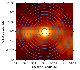
No we can also estimate a radial profile starting from the Galactic center:
[19]:
regions = make_concentric_annulus_sky_regions(
    center=SkyCoord("0d", "0d", frame="galactic"),
    radius_max="1.5 deg",
    nbin=11,
)
Again we first illustrate the regions:
[20]:
geom = RegionGeom.create(region=regions)
gc_image = counts_image.cutout(
    position=SkyCoord("0d", "0d", frame="galactic"), width=3 * u.deg
)
ax = gc_image.smooth("0.1 deg").plot(stretch="sqrt")
geom.plot_region(ax=ax, color="w");
This time we define two energy bins and include the fit statistic profile in the computation:
[21]:
flux_profile_estimator = FluxProfileEstimator(
    regions=regions,
    spectrum=PowerLawSpectralModel(index=2.3),
    energy_edges=[10, 100, 2000] * u.GeV,
    selection_optional=["ul", "scan"],
    norm_values=np.linspace(-1, 5, 11),
)
[22]:
profile = flux_profile_estimator.run(datasets=dataset)
We can directly plot the result:
[23]:
ax = profile.plot(axis_name="projected-distance", sed_type="flux")
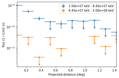
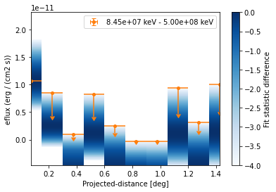
However because of the powerlaw spectrum the flux at high energies is much lower. To extract the profile at high energies only we can use:
[24]:
profile_high = profile.slice_by_idx({"energy": slice(1, 2)})
And now plot the points together with the likelihood profiles:
[25]:
ax = profile_high.plot(sed_type="eflux", color="tab:orange")
profile_high.plot_ts_profiles(ax=ax, sed_type="eflux")
ax.set_yscale("linear")
[ ]: