Statistical utility functions#

gammapy.stats holds statistical estimators, fit statistics and algorithms commonly used in gamma-ray astronomy.

It is mostly concerned with the evaluation of one or several observations that count events in a given region and time window, i.e. with Poisson-distributed counts measurements.

Notations#

For statistical analysis we use the following variable names following mostly the notation in [LiMa1983]. For the MapDataset attributes we chose more verbose equivalents:

Variable	Dataset attribute name	Definition
`n_on`	`counts`	Observed counts
`n_off`	`counts_off`	Observed counts in the off region
`n_bkg`	`background`	Estimated background counts, defined as `alpha * n_off`
`n_sig`	`excess`	Estimated signal counts defined as `n_on` - `n_bkg`
`mu_on`	`npred`	Predicted counts
`mu_off`	`npred_off`	Predicted counts in the off region
`mu_bkg`	`npred_background`	Predicted background counts in the on region
`mu_sig`	`npred_signal`	Predicted signal counts
`a_on`	`acceptance`	Relative background exposure
`a_off`	`acceptance_off`	Relative background exposure in the off region
`alpha`	`alpha`	Background efficiency ratio `a_on` / `a_off`

The on measurement, assumed to contain signal and background counts, $n_{o n}$ follows a Poisson random variable with expected value $μ_{o n} = μ_{s i g} + μ_{b k g}$ .

The off measurement is assumed to contain only background counts, with an acceptance to background $a_{o f f}$ . This off measurement can be used to estimate the number of background counts in the on region: $n_{b k g} = α n_{o f f}$ with $α = a_{o n} / a_{o f f}$ the ratio of on and off acceptances.

Therefore, $n_{o f f}$ follows a Poisson distribution with expected value $μ_{o f f} = μ_{b k g} / α$ .

The expectation or predicted values $μ_{X}$ are in general derived using maximum likelihood estimation.

Counts and fit statistics#

Gamma-ray measurements are counts, $n_{o n}$ , containing both signal and background events.

Estimation of number of signal events or of quantities in physical models is done through Poisson likelihood functions, the fit statistics. In gammapy, they are all log-likelihood functions normalized like chi-squares, i.e. if $L$ is the likelihood function used, they follow the expression $2 \times l o g L$ .

When the expected number of background events, $μ_{b k g}$ is known, the statistic function is Cash (see Cash : Poisson data with background model). When the number of background events is unknown, one has to use a background estimate $n_{b k g}$ taken from an off measurement where only background events are expected. In this case, the statistic function is WStat (see WStat : Poisson data with background measurement).

These statistic functions are at the heart of the model fitting approach in gammapy. They are used to estimate the best fit values of model parameters and their associated confidence intervals.

They are used also to estimate the excess counts significance, i.e. the probability that a given number of measured events $n_{o n}$ actually contains some signal events $n_{s i g}$ , as well as the errors associated to this estimated number of signal counts.

Estimating TS#

A classical approach to modeling and fitting relies on hypothesis testing. One wants to estimate whether an hypothesis $H_{1}$ is statistically preferred over the reference, or null-hypothesis, $H_{0}$ .

The maximum log-likelihood ratio test provides a way to estimate the p-value of the data following $H_{1}$ rather than $H_{0}$ , when the two hypotheses are nested. We note this ratio $λ = \frac{m a x L (X | H_{1})}{m a x L (X | H_{0})}$

The Wilks theorem shows that under some hypothesis, $2 \log λ$ asymptotically follows a $χ^{2}$ distribution with $n_{d o f}$ degrees of freedom, where $n_{d o f}$ is the difference of free parameters between $H_{1}$ and $H_{0}$ .

With the definition the fit statistics $- 2 \log λ$ is simply the difference of the fit statistic values for the two hypotheses, the delta TS (short for test statistic). Hence, $Δ T S$ follows $χ^{2}$ distribution with $n_{d o f}$ degrees of freedom. This can be used to convert $Δ T S$ into a “classical significance” using the following recipe:

from scipy.stats import chi2, norm

def sigma_to_ts(sigma, df=1):
    """Convert sigma to delta ts"""
    p_value = 2 * norm.sf(sigma)
    return chi2.isf(p_value, df=df)

def ts_to_sigma(ts, df=1):
    """Convert delta ts to sigma"""
    p_value = chi2.sf(ts, df=df)
    return norm.isf(0.5 * p_value)

In particular, with only one degree of freedom (e.g. flux amplitude), one can estimate the statistical significance in terms of number of $σ$ as $\sqrt{Δ T S}$ .

In case the excess is negative, which can happen if the background is overestimated the following convention is used:

\begin{array}{r} \sqrt{Δ T S} = {\begin{cases} - \sqrt{Δ T S} & : if Excess < 0 \\ \sqrt{Δ T S} & : else \end{cases} \end{array}

Counts statistics classes#

To estimate the excess counts significance and errors, gammapy uses two classes for Poisson counts with and without known background: CashCountsStatistic and WStatCountsStatistic

We show below how to use them.

Cash counts statistic#

Excess and Significance#

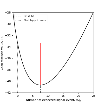
Assume one measured $n_{o n} = 13$ counts in a region where one suspects a source might be present. if the expected number of background events is known (here e.g. $μ_{b k g} = 5.5$ ), one can use the Cash statistic to estimate the signal or excess number, its statistical significance as well as the confidence interval on the true signal counts number value.

from gammapy.stats import CashCountsStatistic
stat = CashCountsStatistic(n_on=13, mu_bkg=5.5)
print(f"Excess  : {stat.n_sig:.2f}")
print(f"Error   : {stat.error:.2f}")
print(f"TS      : {stat.ts:.2f}")
print(f"sqrt(TS): {stat.sqrt_ts:.2f}")
print(f"p-value : {stat.p_value:.4f}")

Excess  : 7.50
Error   : 3.61
TS      : 7.37
sqrt(TS): 2.71
p-value : 0.0033

The error is the symmetric error obtained from the covariance of the statistic function, here $\sqrt{n_{o n}}$ . The sqrt_ts is the square root of the $T S$ , multiplied by the sign of the excess, which is equivalent to the Li & Ma significance for known background. The p-value is now computed taking into account only positive fluctuations.

To see how the $T S$ , relates to the statistic function, we plot below the profile of the Cash statistic as a function of the expected signal events number.

(png, hires.png, pdf)

../../_images/plot_cash_significance.png

Excess errors#

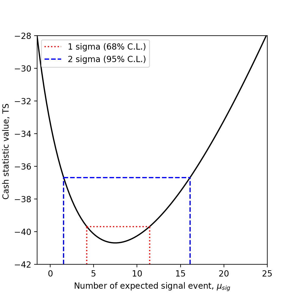
You can also compute the confidence interval for the true excess based on the statistic value: If you are interested in 68% (1 $σ$ ) and 95% (2 $σ$ ) confidence ranges:

from gammapy.stats import CashCountsStatistic
count_statistic = CashCountsStatistic(n_on=13, mu_bkg=5.5)
excess = count_statistic.n_sig
errn = count_statistic.compute_errn(1.)
errp = count_statistic.compute_errp(1.)
print(f"68% confidence range: {excess - errn:.3f} < mu < {excess + errp:.3f}")

68% confidence range: 4.220 < mu < 11.446

errn_2sigma = count_statistic.compute_errn(2.)
errp_2sigma = count_statistic.compute_errp(2.)
print(f"95% confidence range: {excess - errn_2sigma:.3f} < mu < {excess + errp_2sigma:.3f}")

95% confidence range: 1.556 < mu < 16.102

The 68% confidence interval (1 $σ$ ) is obtained by finding the expected signal values for which the TS variation is 1. The 95% confidence interval (2 $σ$ ) is obtained by finding the expected signal values for which the TS variation is $2^{2} = 4$ .

On the following plot, we show how the 1 $σ$ and 2 $σ$ confidence errors relate to the Cash statistic profile.

(png, hires.png, pdf)

WStat counts statistic#

Excess and Significance#

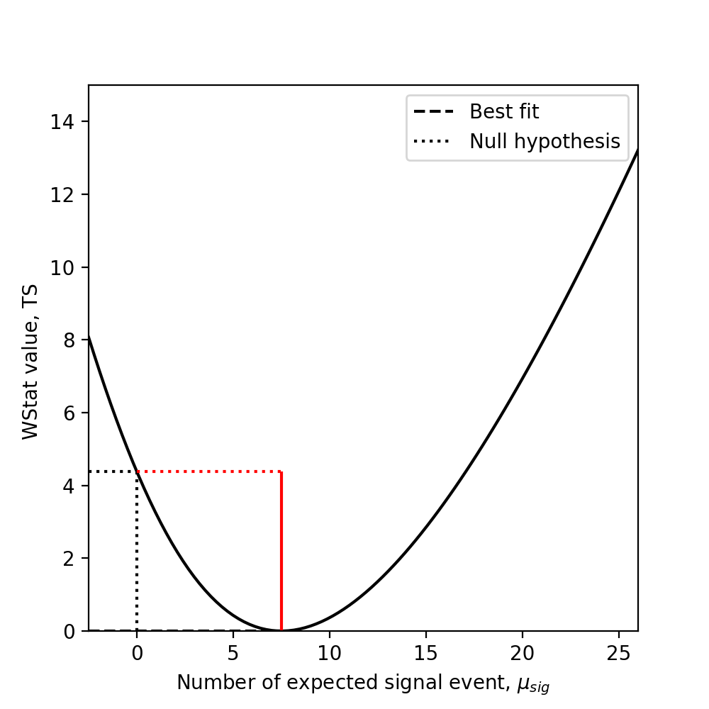
To measure the significance of an excess, one can directly use the TS of the measurement with and without the excess. Taking the square root of the result yields the so-called Li & Ma significance [LiMa1983] (see equation 17).

As an example, assume you measured $n_{o n} = 13$ counts in a region where you suspect a source might be present and $n_{o f f} = 11$ counts in a background control region where you assume no source is present and that is $a_{o f f} / a_{o n} = 2$ times larger than the on-region.

Here’s how you compute the statistical significance of your detection:

from gammapy.stats import WStatCountsStatistic
stat = WStatCountsStatistic(n_on=13, n_off=11, alpha=1./2)
print(f"Excess  : {stat.n_sig:.2f}")
print(f"sqrt(TS): {stat.sqrt_ts:.2f}")

Excess  : 7.50
sqrt(TS): 2.09

(png, hires.png, pdf)

../../_images/plot_wstat_significance.png

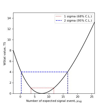
Excess errors#

You can also compute the confidence interval for the true excess based on the statistic value:

If you are interested in 68% (1 $σ$ ) and 95% (1 $σ$ ) confidence errors:

from gammapy.stats import WStatCountsStatistic
count_statistic = WStatCountsStatistic(n_on=13, n_off=11, alpha=1./2)
excess = count_statistic.n_sig
errn = count_statistic.compute_errn(1.)
errp = count_statistic.compute_errp(1.)
print(f"68% confidence range: {excess - errn:.3f} < mu < {excess + errp:.3f}")

68% confidence range: 3.750 < mu < 11.736

errn_2sigma = count_statistic.compute_errn(2.)
errp_2sigma = count_statistic.compute_errp(2.)
print(f"95% confidence range: {excess - errn_2sigma:.3f} < mu < {excess + errp_2sigma:.3f}")

95% confidence range: 0.311 < mu < 16.580

As above, the 68% confidence interval (1 $σ$ ) is obtained by finding the expected signal values for which the TS variation is 1. The 95% confidence interval (2 $σ$ ) is obtained by finding the expected signal values for which the TS variation is $2^{2} = 4$ .

On the following plot, we show how the 1 $σ$ and 2 $σ$ confidence errors relate to the WStat statistic profile.

(png, hires.png, pdf)

These are references describing the available methods: [LiMa1983], [Cash1979], [Stewart2009], [Rolke2005], [Feldman1998], [Cousins2007].