This is a fixed-text formatted version of a Jupyter notebook

• Try online

• You can contribute with your own notebooks in this GitHub repository.

• Source files: analysis_2.ipynb | analysis_2.py

First analysis with gammapy library API

Prerequisites:

• Understanding the gammapy data workflow, in particular what are DL3 events and intrument response functions (IRF).

• Understanding of the data reduction and modeling fitting process as shown in the first gammapy analysis with the high level interface tutorial

Context

This notebook is an introduction to gammapy analysis this time using the lower level classes and functions the library. This allows to understand what happens during two main gammapy analysis steps, data reduction and modeling/fitting.

Objective: Create a 3D dataset of the Crab using the H.E.S.S. DL3 data release 1 and perform a simple model fitting of the Crab nebula using the lower level gammapy API.

Proposed approach:

Here, we have to interact with the data archive (with the gammapy.data.DataStore) to retrieve a list of selected observations (gammapy.data.Observations). Then, we define the geometry of the gammapy.cube.MapDataset object we want to produce and the maker object that reduce an observation to a dataset.

We can then proceed with data reduction with a loop over all selected observations to produce datasets in the relevant geometry and stack them together (i.e. sum them all).

In practice, we have to: - Create a gammapy.data.DataStore poiting to the relevant data - Apply an observation selection to produce a list of observations, a gammapy.data.Observations object. - Define a geometry of the Map we want to produce, with a sky projection and an energy range. - Create a gammapy.maps.MapAxis for the energy - Create a gammapy.maps.WcsGeom for the geometry - Create the necessary makers : - the map dataset maker : gammapy.cube.MapDatasetMaker - the background normalization maker, here a gammapy.cube.FoVBackgroundMaker - and usually the safe range maker : gammapy.cube.SafeRangeMaker - Perform the data reduction loop. And for every observation: - Apply the makers sequentially to produce the current gammapy.maps.MapDataset - Stack it on the target one. - Define the gammapy.modeling.models.SkyModel to apply to the dataset. - Create a gammapy.modeling.Fit object and run it to fit the model parameters - Apply a gammapy.spectrum.FluxPointsEstimator to compute flux points for the spectral part of the fit.

Setup

First, we setup the analysis by performing required imports.

%matplotlib inline
import matplotlib.pyplot as plt

from pathlib import Path
import numpy as np
from astropy import units as u
from astropy.coordinates import SkyCoord
from regions import CircleSkyRegion

from gammapy.data import DataStore
from gammapy.maps import WcsGeom, MapAxis, Map
from gammapy.cube import (
    MapDatasetMaker,
    MapDataset,
    SafeMaskMaker,
    FoVBackgroundMaker,
)
from gammapy.modeling.models import (
    SkyModel,
    PowerLawSpectralModel,
    PointSpatialModel,
)
from gammapy.modeling import Fit
from gammapy.spectrum import FluxPointsEstimator

Defining the datastore and selecting observations

We first use the gammapy.data.DataStore object to access the observations we want to analyse. Here the H.E.S.S. DL3 DR1.

data_store = DataStore.from_dir("$GAMMAPY_DATA/hess-dl3-dr1")

We can now define an observation filter to select only the relevant observations. Here we use a cone search which we define with a python dict.

We then filter the ObservationTable with gammapy.data.ObservationTable.select_observations().

selection = dict(
    type="sky_circle",
    frame="icrs",
    lon="83.633 deg",
    lat="22.014 deg",
    radius="5 deg",
)
selected_obs_table = data_store.obs_table.select_observations(selection)

We can now retrieve the relevant observations by passing their obs_id to thegammapy.data.DataStore.get_observations() method.

observations = data_store.get_observations(selected_obs_table["OBS_ID"])

Preparing reduced datasets geometry

Now we define a reference geometry for our analysis, We choose a WCS based geometry with a binsize of 0.02 deg and also define an energy axis:

energy_axis = MapAxis.from_energy_bounds(1.0, 10.0, 4, unit="TeV")

geom = WcsGeom.create(
    skydir=(83.633, 22.014),
    binsz=0.02,
    width=(2, 2),
    frame="icrs",
    proj="CAR",
    axes=[energy_axis],
)

# Reduced IRFs are defined in true energy (i.e. not measured energy).
energy_axis_true = MapAxis.from_energy_bounds(0.5, 20, 10, unit="TeV")

Now we can define the target dataset with this geometry.

stacked = MapDataset.create(
    geom=geom, energy_axis_true=energy_axis_true, name="crab-stacked"
)

Data reduction

Create the maker classes to be used

The gammapy.cube.MapDatasetMaker object is initialized as well as the gammapy.cube.SafeMaskMaker that carries here a maximum offset selection.

offset_max = 2.5 * u.deg
maker = MapDatasetMaker()
maker_safe_mask = SafeMaskMaker(methods=["offset-max"], offset_max=offset_max)

circle = CircleSkyRegion(
    center=SkyCoord("83.63 deg", "22.14 deg"), radius=0.2 * u.deg
)
data = geom.region_mask(regions=[circle], inside=False)
exclusion_mask = Map.from_geom(geom=geom, data=data)
maker_fov = FoVBackgroundMaker(method="fit", exclusion_mask=exclusion_mask)

Perform the data reduction loop

%%time

for obs in observations:
    # First a cutout of the target map is produced
    cutout = stacked.cutout(obs.pointing_radec, width=2 * offset_max)
    # A MapDataset is filled in this cutout geometry
    dataset = maker.run(cutout, obs)
    # fit background model
    dataset = maker_fov.run(dataset)
    print(
        f"Background norm obs {obs.obs_id}: {dataset.background_model.norm.value:.2f}"
    )
    # The data quality cut is applied
    dataset = maker_safe_mask.run(dataset, obs)
    # The resulting dataset cutout is stacked onto the final one
    stacked.stack(dataset)

Background norm obs 23523: 0.99
Background norm obs 23526: 1.08
Background norm obs 23559: 0.98
Background norm obs 23592: 1.09
CPU times: user 1.78 s, sys: 102 ms, total: 1.88 s
Wall time: 1.91 s

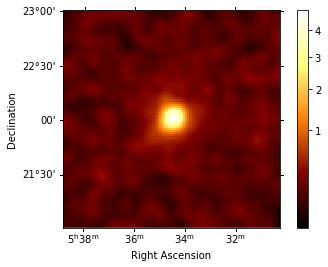
Inspect the reduced dataset

stacked.counts.sum_over_axes().smooth(0.05 * u.deg).plot(
    stretch="sqrt", add_cbar=True
)

(<Figure size 432x288 with 2 Axes>,
 <matplotlib.axes._subplots.WCSAxesSubplot at 0x1c1d3c9c88>,
 <matplotlib.colorbar.Colorbar at 0x1c1d4e3da0>)

Save dataset to disk

It is common to run the preparation step independent of the likelihood fit, because often the preparation of maps, PSF and energy dispersion is slow if you have a lot of data. We first create a folder:

path = Path("analysis_2")
path.mkdir(exist_ok=True)

And then write the maps and IRFs to disk by calling the dedicated gammapy.cube.MapDataset.write() method:

filename = path / "crab-stacked-dataset.fits.gz"
stacked.write(filename, overwrite=True)

Define the model

We first define the model, a SkyModel, as the combination of a point source SpatialModel with a powerlaw SpectralModel:

target_position = SkyCoord(ra=83.63308, dec=22.01450, unit="deg")
spatial_model = PointSpatialModel(
    lon_0=target_position.ra, lat_0=target_position.dec, frame="icrs"
)

spectral_model = PowerLawSpectralModel(
    index=2.702,
    amplitude=4.712e-11 * u.Unit("1 / (cm2 s TeV)"),
    reference=1 * u.TeV,
)

sky_model = SkyModel(
    spatial_model=spatial_model, spectral_model=spectral_model, name="crab"
)

Now we assign this model to our reduced dataset:

stacked.models = sky_model

Fit the model

The gammapy.modeling.Fit class is orchestrating the fit, connecting the stats method of the dataset to the minimizer. By default, it uses iminuit.

Its contructor takes a list of dataset as argument.

%%time
fit = Fit([stacked])
result = fit.run(optimize_opts={"print_level": 1})

------------------------------------------------------------------
| FCN = 1.624E+04               |     Ncalls=137 (137 total)     |
| EDM = 5.25E-05 (Goal: 1E-05)  |            up = 1.0            |
------------------------------------------------------------------
|  Valid Min.   | Valid Param.  | Above EDM | Reached call limit |
------------------------------------------------------------------
|     True      |     True      |   False   |       False        |
------------------------------------------------------------------
| Hesse failed  |   Has cov.    | Accurate  | Pos. def. | Forced |
------------------------------------------------------------------
|     False     |     True      |   True    |   True    | False  |
------------------------------------------------------------------
CPU times: user 3.08 s, sys: 134 ms, total: 3.22 s
Wall time: 3.27 s

The FitResult contains information on the fitted parameters.

result.parameters.to_table()

Table length=8

name	value	error	unit	min	max	frozen
str9	float64	float64	str14	float64	float64	bool
lon_0	8.362e+01	3.116e-03	deg	nan	nan	False
lat_0	2.202e+01	2.965e-03	deg	-9.000e+01	9.000e+01	False
index	2.595e+00	1.000e-01		nan	nan	False
amplitude	4.590e-11	3.757e-12	cm-2 s-1 TeV-1	nan	nan	False
reference	1.000e+00	0.000e+00	TeV	nan	nan	True
norm	9.370e-01	2.198e-02		0.000e+00	nan	False
tilt	0.000e+00	0.000e+00		nan	nan	True
reference	1.000e+00	0.000e+00	TeV	nan	nan	True

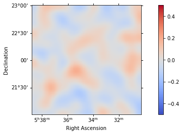
Inspecting residuals

For any fit it is usefull to inspect the residual images. We have a few option on the dataset object to handle this. First we can use .plot_residuals() to plot a residual image, summed over all energies:

stacked.plot_residuals(method="diff/sqrt(model)", vmin=-0.5, vmax=0.5)

(<matplotlib.axes._subplots.WCSAxesSubplot at 0x1c1d761400>, None)

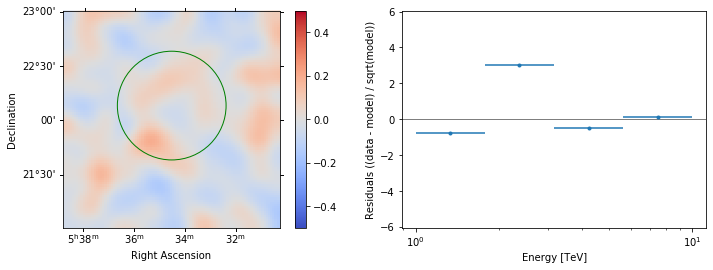
In addition we can aslo specify a region in the map to show the spectral residuals:

region = CircleSkyRegion(
    center=SkyCoord("83.63 deg", "22.14 deg"), radius=0.5 * u.deg
)

stacked.plot_residuals(
    region=region, method="diff/sqrt(model)", vmin=-0.5, vmax=0.5
)

(<matplotlib.axes._subplots.WCSAxesSubplot at 0x1c1fd84780>,
 <matplotlib.axes._subplots.AxesSubplot at 0x1c1fc93160>)

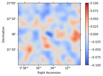
We can also directly access the .residuals() to get a map, that we can plot interactively:

residuals = stacked.residuals(method="diff")
residuals.smooth("0.08 deg").plot_interactive(
    cmap="coolwarm", vmin=-0.1, vmax=0.1, stretch="linear", add_cbar=True
)

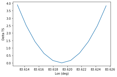
Inspecting fit statistic profiles

To check the quality of the fit it is also useful to plot fit statistic profiles for specific parameters. For this we use gammapy.modeling.Fit.stat_profile().

profile = fit.stat_profile(parameter="lon_0")

For a good fit and error estimate the profile should be parabolic, if we plot it:

total_stat = result.total_stat
plt.plot(profile["values"], profile["stat"] - total_stat)
plt.xlabel("Lon (deg)")
plt.ylabel("Delta TS")

Text(0, 0.5, 'Delta TS')

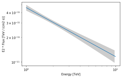
Plot the fitted spectrum

Making a butterfly plot

The SpectralModel component can be used to produce a, so-called, butterfly plot showing the enveloppe of the model taking into account parameter uncertainties.

To do so, we have to copy the part of the covariance matrix stored on the FitResult on the model parameters:

spec = sky_model.spectral_model

# set covariance on the spectral model
covar = result.parameters.get_subcovariance(spec.parameters)
spec.parameters.covariance = covar

Now we can actually do the plot using the plot_error method:

energy_range = [1, 10] * u.TeV
spec.plot(energy_range=energy_range, energy_power=2)
ax = spec.plot_error(energy_range=energy_range, energy_power=2)

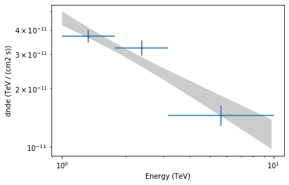
Computing flux points

We can now compute some flux points using the gammapy.spectrum.FluxPointsEstimator.

Besides the list of datasets to use, we must provide it the energy intervals on which to compute flux points as well as the model component name.

e_edges = [1, 2, 4, 10] * u.TeV
fpe = FluxPointsEstimator(datasets=[stacked], e_edges=e_edges, source="crab")

%%time
flux_points = fpe.run()

CPU times: user 1.78 s, sys: 42.7 ms, total: 1.83 s
Wall time: 1.85 s

ax = spec.plot_error(energy_range=energy_range, energy_power=2)
flux_points.plot(ax=ax, energy_power=2)

<matplotlib.axes._subplots.AxesSubplot at 0x1c1bbbc710>