This is a fixed-text formatted version of a Jupyter notebook
Try online

You can contribute with your own notebooks in this GitHub repository.
Source files: detect.ipynb | detect.py
Source detection with Gammapy
Context
The first task in a source catalogue production is to identify significant excesses in the data that can be associated to unknown sources and provide a preliminary parametrization in term of position, extent, and flux. In this notebook we will use Fermi-LAT data to illustrate how to detect candidate sources in counts images with known background.
Objective: build a list of significant excesses in a Fermi-LAT map
Proposed approach
This notebook show how to do source detection with Gammapy using the methods available in gammapy.detect. We will use images from a Fermi-LAT 3FHL high-energy Galactic center dataset to do this:
perform adaptive smoothing on counts image
produce 2-dimensional test-statistics (TS)
run a peak finder to detect point-source candidates
compute Li & Ma significance images
estimate source candidates radius and excess counts
Note that what we do here is a quick-look analysis, the production of real source catalogs use more elaborate procedures.
We will work with the following functions and classes:
Setup
As always, let’s get started with some setup …
[1]:
%matplotlib inline
import matplotlib.pyplot as plt
import matplotlib.cm as cm
from gammapy.maps import Map
from gammapy.detect import (
    ASmoothMapEstimator,
    TSMapEstimator,
    find_peaks,
    compute_lima_image,
)
from gammapy.catalog import SOURCE_CATALOGS
from gammapy.modeling.models import BackgroundModel
from gammapy.cube import PSFKernel, MapDataset
from gammapy.stats import significance
from astropy.coordinates import SkyCoord
from astropy.convolution import Tophat2DKernel
import astropy.units as u
import numpy as np
Read in input images
We first read in the counts cube and sum over the energy axis:
[2]:
counts = Map.read(
    "$GAMMAPY_DATA/fermi-3fhl-gc/fermi-3fhl-gc-counts-cube.fits.gz"
)
background = Map.read(
    "$GAMMAPY_DATA/fermi-3fhl-gc/fermi-3fhl-gc-background-cube.fits.gz"
)
background = BackgroundModel(background)

exposure = Map.read(
    "$GAMMAPY_DATA/fermi-3fhl-gc/fermi-3fhl-gc-exposure-cube.fits.gz"
)
mask_safe = counts.copy(data=np.ones_like(counts.data).astype("bool"))

dataset = MapDataset(
    counts=counts,
    background_model=background,
    exposure=exposure,
    mask_safe=mask_safe,
)

dataset = dataset.to_image()
WARNING: FITSFixedWarning: 'datfix' made the change 'Set DATE-REF to '1858-11-17' from MJD-REF.
Set MJD-OBS to 54682.655278 from DATE-OBS.
Set MJD-END to 57236.967546 from DATE-END'. [astropy.wcs.wcs]
WARNING: FITSFixedWarning: 'datfix' made the change 'Set DATE-REF to '2001-01-01T00:01:04.184' from MJD-REF.
Set MJD-OBS to 54682.655283 from DATE-OBS.
Set MJD-END to 57236.967546 from DATE-END'. [astropy.wcs.wcs]
[3]:
kernel = PSFKernel.read(
    "$GAMMAPY_DATA/fermi-3fhl-gc/fermi-3fhl-gc-psf.fits.gz"
)
WARNING: FITSFixedWarning: 'datfix' made the change 'Set DATE-REF to '1858-11-17' from MJD-REF'. [astropy.wcs.wcs]
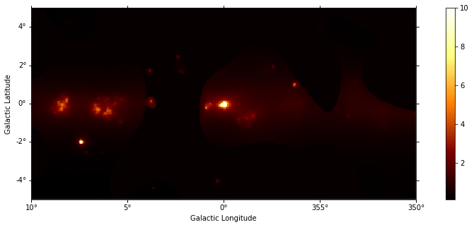
Adaptive smoothing
For visualisation purpose it can be nice to look at a smoothed counts image. This can be performed using the adaptive smoothing algorithm from Ebeling et al. (2006).
In the following example the threshold argument gives the minimum significance expected, values below are clipped.
[4]:
%%time
scales = u.Quantity(np.arange(0.05, 1, 0.05), unit="deg")
smooth = ASmoothMapEstimator(threshold=3, scales=scales)
images = smooth.run(dataset)

plt.figure(figsize=(15, 5))
images["counts"].plot(add_cbar=True, vmax=10)
/Users/adonath/github/adonath/gammapy/gammapy/maps/image_utils.py:46: FutureWarning: arrays to stack must be passed as a "sequence" type such as list or tuple. Support for non-sequence iterables such as generators is deprecated as of NumPy 1.16 and will raise an error in the future.
  return np.dstack(_fftconvolve_wrap(kernel, data) for kernel in kernels)
CPU times: user 1.06 s, sys: 443 ms, total: 1.5 s
Wall time: 1.53 s
[4]:
(<Figure size 1080x360 with 2 Axes>,
 <matplotlib.axes._subplots.WCSAxesSubplot at 0x1c145404e0>,
 <matplotlib.colorbar.Colorbar at 0x1c159bd940>)
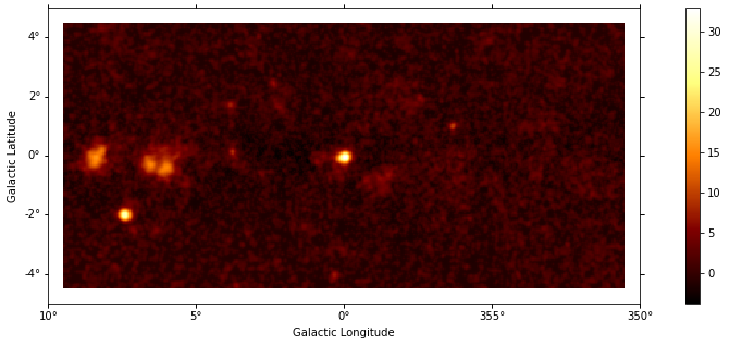
TS map estimation
The Test Statistic, TS = 2 ∆ log L (Mattox et al. 1996), compares the likelihood function L optimized with and without a given source. The TS map is computed by fitting by a single amplitude parameter on each pixel as described in Appendix A of Stewart (2009). The fit is simplified by finding roots of the derivative of the fit statistics (default settings use Brent’s method).
[5]:
%%time
estimator = TSMapEstimator()
images = estimator.run(dataset, kernel.data)
CPU times: user 8.95 s, sys: 176 ms, total: 9.12 s
Wall time: 9.27 s
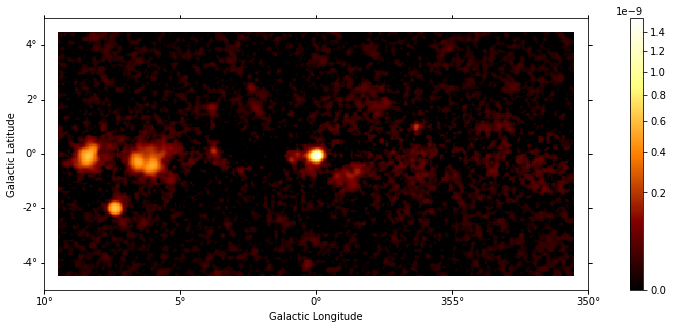
Plot resulting images
[6]:
plt.figure(figsize=(15, 5))
images["sqrt_ts"].plot(add_cbar=True);
[7]:
plt.figure(figsize=(15, 5))
images["flux"].plot(add_cbar=True, stretch="sqrt", vmin=0);
/Users/adonath/software/anaconda3/envs/gammapy-dev/lib/python3.7/site-packages/matplotlib/colors.py:527: RuntimeWarning: invalid value encountered in less
  xa[xa < 0] = -1
/Users/adonath/software/anaconda3/envs/gammapy-dev/lib/python3.7/site-packages/matplotlib/colors.py:527: RuntimeWarning: invalid value encountered in less
  xa[xa < 0] = -1
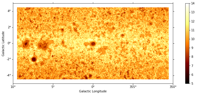
[8]:
plt.figure(figsize=(15, 5))
images["niter"].plot(add_cbar=True);
Source candidates
Let’s run a peak finder on the sqrt_ts image to get a list of point-sources candidates (positions and peak sqrt_ts values). The find_peaks function performs a local maximun search in a sliding window, the argument min_distance is the minimum pixel distance between peaks (smallest possible value and default is 1 pixel).
[9]:
sources = find_peaks(images["sqrt_ts"], threshold=8, min_distance=1)
nsou = len(sources)
sources
[9]:
| value | x | y | ra | dec |
|---|---|---|---|---|
| deg | deg | |||
| float64 | int64 | int64 | float64 | float64 |
| 32.972 | 200 | 99 | 266.41449 | -28.97054 |
| 27.995 | 52 | 60 | 272.43197 | -23.54282 |
| 16.18 | 32 | 98 | 271.16056 | -21.74479 |
| 14.939 | 69 | 93 | 270.40919 | -23.47797 |
| 14.842 | 80 | 92 | 270.15899 | -23.98049 |
| 13.951 | 36 | 102 | 270.86716 | -21.82076 |
| 9.7246 | 273 | 119 | 263.18257 | -31.52587 |
| 8.8532 | 124 | 102 | 268.46711 | -25.63326 |
[10]:
# Plot sources on top of significance sky image
plt.figure(figsize=(15, 5))

_, ax, _ = images["sqrt_ts"].plot(add_cbar=True)

ax.scatter(
    sources["ra"],
    sources["dec"],
    transform=plt.gca().get_transform("icrs"),
    color="none",
    edgecolor="w",
    marker="o",
    s=600,
    lw=1.5,
);
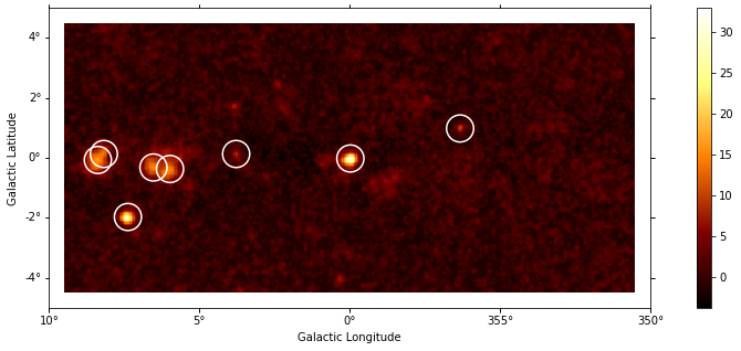
Note that we used the instrument point-spread-function (PSF) as kernel, so the hypothesis we test is the presence of a point source. In order to test for extended sources we would have to use as kernel an extended template convolved by the PSF. Alternatively, we can compute the significance of an extended excess using the Li & Ma formalism, which is faster as no fitting is involve.
What next?
In this notebook, we have seen how to work with images and compute TS and significance images from counts data, if a background estimate is already available.
Here’s some suggestions what to do next:
Look how background estimation is performed for IACTs with and without the high-level interface in analysis_1 and analysis_2 notebooks, respectively
Learn about 2D model fitting in the modeling 2D notebook
find more about Fermi-LAT data analysis in the fermi_lat notebook
Use source candidates to build a model and perform a 3D fitting (see analysis_3d, analysis_mwl notebooks for some hints)
[ ]: