This is a fixed-text formatted version of a Jupyter notebook
Try online

You may download all the notebooks as a tar file.
Source files: fermi_lat.ipynb | fermi_lat.py
Fermi-LAT with Gammapy#
Introduction#
This tutorial will show you how to work with Fermi-LAT data with Gammapy. As an example, we will look at the Galactic center region using the high-energy dataset that was used for the 3FHL catalog, in the energy range 10 GeV to 2 TeV.
We note that support for Fermi-LAT data analysis in Gammapy is very limited. For most tasks, we recommend you use Fermipy, which is based on the Fermi Science Tools (Fermi ST).
Using Gammapy with Fermi-LAT data could be an option for you if you want to do an analysis that is not easily possible with Fermipy and the Fermi Science Tools. For example a joint likelihood fit of Fermi-LAT data with data e.g. from H.E.S.S., MAGIC, VERITAS or some other instrument, or analysis of Fermi-LAT data with a complex spatial or spectral model that is not available in Fermipy or the Fermi ST.
Besides Gammapy, you might want to look at are Sherpa or 3ML. Or just using Python to roll your own analysis using several existing analysis packages. E.g. it it possible to use Fermipy and the Fermi ST to evaluate the likelihood on Fermi-LAT data, and Gammapy to evaluate it e.g. for IACT data, and to do a joint likelihood fit using e.g. iminuit or emcee.
To use Fermi-LAT data with Gammapy, you first have to use the Fermi ST to prepare an event list (using gtselect and gtmktime, exposure cube (using gtexpcube2 and PSF (using gtpsf). You can then use gammapy.data.EventList, ~gammapy.maps and the gammapy.irf.PSFMap to read the Fermi-LAT maps and PSF, i.e. support for these high level analysis products from the Fermi ST is built in. To do a 3D map analysis, you can use Fit for Fermi-LAT data in the same way that it’s
use for IACT data. This is illustrated in this notebook. A 1D region-based spectral analysis is also possible, this will be illustrated in a future tutorial.
Setup#
IMPORTANT: For this notebook you have to get the prepared 3fhl dataset provided in your $GAMMAPY_DATA.
Note that the 3fhl dataset is high-energy only, ranging from 10 GeV to 2 TeV.
[1]:
# Check that you have the prepared Fermi-LAT dataset
# We will use diffuse models from here
!ls -1 $GAMMAPY_DATA/fermi_3fhl
fermi_3fhl_events_selected.fits.gz
fermi_3fhl_exposure_cube_hpx.fits.gz
fermi_3fhl_psf_gc.fits.gz
gll_iem_v06_cutout.fits
iso_P8R2_SOURCE_V6_v06.txt
[2]:
%matplotlib inline
import matplotlib.pyplot as plt
[3]:
from astropy import units as u
from astropy.coordinates import SkyCoord
from gammapy.data import EventList
from gammapy.datasets import MapDataset
from gammapy.irf import PSFMap, EDispKernelMap
from gammapy.maps import Map, MapAxis, WcsGeom
from gammapy.modeling.models import (
    PowerLawSpectralModel,
    PointSpatialModel,
    SkyModel,
    TemplateSpatialModel,
    PowerLawNormSpectralModel,
    Models,
    create_fermi_isotropic_diffuse_model,
)
from gammapy.modeling import Fit
Events#
To load up the Fermi-LAT event list, use the gammapy.data.EventList class:
[4]:
events = EventList.read(
    "$GAMMAPY_DATA/fermi_3fhl/fermi_3fhl_events_selected.fits.gz"
)
print(events)
EventList
---------

  Instrument       : LAT
  Telescope        : GLAST
  Obs. ID          :

  Number of events : 697317
  Event rate       : 0.003 1 / s

  Time start       : 54682.65603222222
  Time stop        : 57236.96833546296

  Min. energy      : 1.00e+04 MeV
  Max. energy      : 2.00e+06 MeV
  Median energy    : 1.59e+04 MeV
The event data is stored in a astropy.table.Table object. In case of the Fermi-LAT event list this contains all the additional information on position, zenith angle, earth azimuth angle, event class, event type etc.
[5]:
events.table.colnames
[5]:
['ENERGY',
 'RA',
 'DEC',
 'L',
 'B',
 'THETA',
 'PHI',
 'ZENITH_ANGLE',
 'EARTH_AZIMUTH_ANGLE',
 'TIME',
 'EVENT_ID',
 'RUN_ID',
 'RECON_VERSION',
 'CALIB_VERSION',
 'EVENT_CLASS',
 'EVENT_TYPE',
 'CONVERSION_TYPE',
 'LIVETIME',
 'DIFRSP0',
 'DIFRSP1',
 'DIFRSP2',
 'DIFRSP3',
 'DIFRSP4']
[6]:
events.table[:5][["ENERGY", "RA", "DEC"]]
[6]:
| ENERGY | RA | DEC |
|---|---|---|
| MeV | deg | deg |
| float32 | float32 | float32 |
| 12856.5205 | 139.64438 | -9.93702 |
| 14773.319 | 177.04454 | 60.55275 |
| 23273.527 | 110.21325 | 37.002018 |
| 41866.125 | 334.85287 | 17.577398 |
| 42463.074 | 316.86676 | 48.152477 |
[7]:
print(events.time[0].iso)
print(events.time[-1].iso)
2008-08-04 15:49:26.782
2015-07-30 11:00:41.226
[8]:
energy = events.energy
energy.info("stats")
name = ENERGY
mean = 28905.5 MeV
std = 61051.7 MeV
min = 10000 MeV
max = 1.99848e+06 MeV
n_bad = 0
length = 697317
As a short analysis example we will count the number of events above a certain minimum energy:
[9]:
for e_min in [10, 100, 1000] * u.GeV:
    n = (events.energy > e_min).sum()
    print(f"Events above {e_min:4.0f}: {n:5.0f}")
Events above   10 GeV: 697317
Events above  100 GeV: 23628
Events above 1000 GeV:   544
Counts#
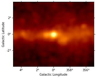
Let us start to prepare things for an 3D map analysis of the Galactic center region with Gammapy. The first thing we do is to define the map geometry. We chose a TAN projection centered on position (glon, glat) = (0, 0) with pixel size 0.1 deg, and four energy bins.
[10]:
gc_pos = SkyCoord(0, 0, unit="deg", frame="galactic")
energy_axis = MapAxis.from_edges(
    [1e4, 3e4, 1e5, 3e5, 2e6], name="energy", unit="MeV", interp="log"
)
counts = Map.create(
    skydir=gc_pos,
    npix=(100, 80),
    proj="TAN",
    frame="galactic",
    binsz=0.1,
    axes=[energy_axis],
    dtype=float,
)
# We put this call into the same Jupyter cell as the Map.create
# because otherwise we could accidentally fill the counts
# multiple times when executing the ``fill_by_coord`` multiple times.
counts.fill_events(events)
[11]:
counts.geom.axes[0]
[11]:
MapAxis

        name       : energy
        unit       : 'MeV'
        nbins      : 4
        node type  : edges
        edges min  : 1.0e+04 MeV
        edges max  : 2.0e+06 MeV
        interp     : log
[12]:
counts.sum_over_axes().smooth(2).plot(stretch="sqrt", vmax=30);
Exposure#
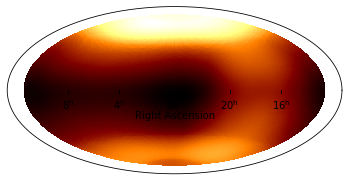
The Fermi-LAT dataset contains the energy-dependent exposure for the whole sky as a HEALPix map computed with gtexpcube2. This format is supported by ~gammapy.maps directly.
Interpolating the exposure cube from the Fermi ST to get an exposure cube matching the spatial geometry and energy axis defined above with Gammapy is easy. The only point to watch out for is how exactly you want the energy axis and binning handled.
Below we just use the default behaviour, which is linear interpolation in energy on the original exposure cube. Probably log interpolation would be better, but it doesn’t matter much here, because the energy binning is fine. Finally, we just copy the counts map geometry, which contains an energy axis with node_type="edges". This is non-ideal for exposure cubes, but again, acceptable because exposure doesn’t vary much from bin to bin, so the exact way interpolation occurs in later use of that
exposure cube doesn’t matter a lot. Of course you could define any energy axis for your exposure cube that you like.
[13]:
exposure_hpx = Map.read(
    "$GAMMAPY_DATA/fermi_3fhl/fermi_3fhl_exposure_cube_hpx.fits.gz"
)
print(exposure_hpx.geom)
print(exposure_hpx.geom.axes[0])
HpxGeom

        axes       : ['skycoord', 'energy_true']
        shape      : (49152, 18)
        ndim       : 3
        nside      : 64
        nested     : False
        frame      : icrs
        projection : HPX
        center     : 0.0 deg, 0.0 deg

MapAxis

        name       : energy_true
        unit       : 'MeV'
        nbins      : 18
        node type  : center
        center min : 1.0e+04 MeV
        center max : 2.0e+06 MeV
        interp     : log
WARNING: version mismatch between CFITSIO header (v4.000999999999999) and linked library (v4.01).


WARNING: version mismatch between CFITSIO header (v4.000999999999999) and linked library (v4.01).


WARNING: version mismatch between CFITSIO header (v4.000999999999999) and linked library (v4.01).
[14]:
exposure_hpx.plot();
[15]:
# For exposure, we choose a geometry with node_type='center',
# whereas for counts it was node_type='edge'
axis = MapAxis.from_energy_bounds(
    "10 GeV",
    "2 TeV",
    nbin=10,
    per_decade=True,
    name="energy_true",
)
geom = WcsGeom(wcs=counts.geom.wcs, npix=counts.geom.npix, axes=[axis])

exposure = exposure_hpx.interp_to_geom(geom)
[16]:
counts.geom.axes[0]
[16]:
MapAxis

        name       : energy
        unit       : 'MeV'
        nbins      : 4
        node type  : edges
        edges min  : 1.0e+04 MeV
        edges max  : 2.0e+06 MeV
        interp     : log
[17]:
print(exposure.geom)
print(exposure.geom.axes[0])
WcsGeom

        axes       : ['lon', 'lat', 'energy_true']
        shape      : (100, 80, 24)
        ndim       : 3
        frame      : galactic
        projection : TAN
        center     : 0.0 deg, 0.0 deg
        width      : 10.0 deg x 8.0 deg
        wcs ref    : 0.0 deg, 0.0 deg

MapAxis

        name       : energy_true
        unit       : 'TeV'
        nbins      : 24
        node type  : edges
        edges min  : 1.0e-02 TeV
        edges max  : 2.0e+00 TeV
        interp     : log
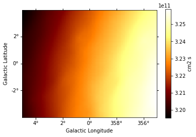
[18]:
# Exposure is almost constant across the field of view
exposure.slice_by_idx({"energy_true": 0}).plot(add_cbar=True);
[19]:
# Exposure varies very little with energy at these high energies
energy = [10, 100, 1000] * u.GeV
exposure.get_by_coord({"skycoord": gc_pos, "energy_true": energy})
[19]:
array([3.22974080e+11, 3.29585273e+11, 2.90605275e+11])
Galactic diffuse background#
The Fermi-LAT collaboration provides a galactic diffuse emission model, that can be used as a background model for Fermi-LAT source analysis.
Diffuse model maps are very large (100s of MB), so as an example here, we just load one that represents a small cutout for the Galactic center region.
[20]:
diffuse_galactic_fermi = Map.read(
    "$GAMMAPY_DATA/fermi-3fhl-gc/gll_iem_v06_gc.fits.gz"
)

print(diffuse_galactic_fermi)

print(diffuse_galactic_fermi.geom.axes[0])
WcsNDMap

        geom  : WcsGeom
        axes  : ['lon', 'lat', 'energy_true']
        shape : (120, 64, 30)
        ndim  : 3
        unit  : 1 / (cm2 MeV s sr)
        dtype : >f4

MapAxis

        name       : energy_true
        unit       : 'MeV'
        nbins      : 30
        node type  : center
        center min : 5.8e+01 MeV
        center max : 5.1e+05 MeV
        interp     : log
[21]:
template_diffuse = TemplateSpatialModel(
    diffuse_galactic_fermi, normalize=False
)
[22]:
diffuse_iem = SkyModel(
    spectral_model=PowerLawNormSpectralModel(),
    spatial_model=template_diffuse,
    name="diffuse-iem",
)
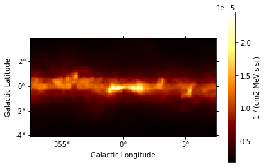
Let’s look at the map of first energy band of the cube:
[23]:
template_diffuse.map.slice_by_idx({"energy_true": 0}).plot(add_cbar=True);
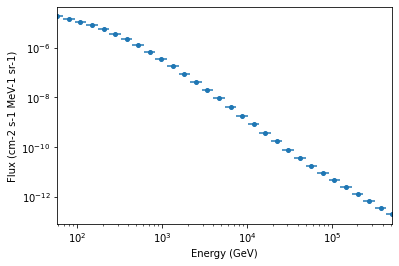
Here is the spectrum at the Glaactic center:
[24]:
dnde = template_diffuse.map.to_region_nd_map(region=gc_pos)
dnde.plot()
plt.xlabel("Energy (GeV)")
plt.ylabel("Flux (cm-2 s-1 MeV-1 sr-1)");
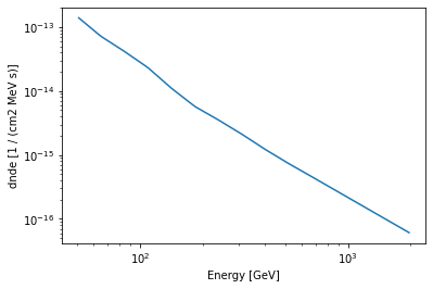
Isotropic diffuse background#
To load the isotropic diffuse model with Gammapy, use the gammapy.modeling.models.TemplateSpectralModel. We are using 'fill_value': 'extrapolate' to extrapolate the model above 500 GeV:
[25]:
filename = "$GAMMAPY_DATA/fermi_3fhl/iso_P8R2_SOURCE_V6_v06.txt"

diffuse_iso = create_fermi_isotropic_diffuse_model(
    filename=filename, interp_kwargs={"fill_value": None}
)
We can plot the model in the energy range between 50 GeV and 2000 GeV:
[26]:
energy_bounds = [50, 2000] * u.GeV
diffuse_iso.spectral_model.plot(
    energy_bounds, yunits=u.Unit("1 / (cm2 MeV s)")
);
PSF#
Next we will tke a look at the PSF. It was computed using gtpsf, in this case for the Galactic center position. Note that generally for Fermi-LAT, the PSF only varies little within a given regions of the sky, especially at high energies like what we have here. We use the gammapy.irf.PSFMap class to load the PSF and use some of it’s methods to get some information about it.
[27]:
psf = PSFMap.read(
    "$GAMMAPY_DATA/fermi_3fhl/fermi_3fhl_psf_gc.fits.gz", format="gtpsf"
)
print(psf)
RegionNDMap

        geom  : RegionGeom
        axes  : ['lon', 'lat', 'rad', 'energy_true']
        shape : (1, 1, 300, 17)
        ndim  : 4
        unit  : 1 / sr
        dtype : >f8
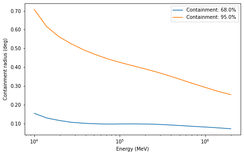
To get an idea of the size of the PSF we check how the containment radii of the Fermi-LAT PSF vari with energy and different containment fractions:
[28]:
plt.figure(figsize=(8, 5))
psf.plot_containment_radius_vs_energy()
plt.show()
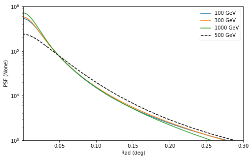
In addition we can check how the actual shape of the PSF varies with energy and compare it against the mean PSF between 50 GeV and 2000 GeV:
[29]:
plt.figure(figsize=(8, 5))

energy = [100, 300, 1000] * u.GeV
psf.plot_psf_vs_rad(energy_true=energy)

spectrum = PowerLawSpectralModel(index=2.3)
psf_mean = psf.to_image(spectrum=spectrum)
psf_mean.plot_psf_vs_rad(c="k", ls="--", energy_true=[500] * u.GeV)

plt.xlim(1e-3, 0.3)
plt.ylim(1e3, 1e6)
plt.legend();
[30]:
psf_kernel = psf.get_psf_kernel(
position=geom.center_skydir, geom=geom, max_radius="1 deg"
)
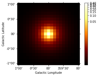
psf_kernel.to_image().psf_kernel_map.plot(stretch="log", add_cbar=True);
Energy Dispersion#
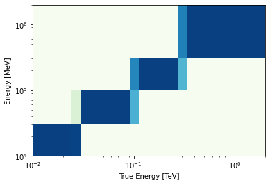
For simplicity we assume a diagonal energy dispersion:
[31]:
e_true = exposure.geom.axes["energy_true"]
edisp = EDispKernelMap.from_diagonal_response(
    energy_axis_true=e_true, energy_axis=energy_axis
)
[32]:
edisp.get_edisp_kernel().plot_matrix()
[32]:
<AxesSubplot:xlabel='True Energy [TeV]', ylabel='Energy [MeV]'>
Fit#
Now, the big finale: let’s do a 3D map fit for the source at the Galactic center, to measure it’s position and spectrum. We keep the background normalization free.
[33]:
spatial_model = PointSpatialModel(
    lon_0="0 deg", lat_0="0 deg", frame="galactic"
)
spectral_model = PowerLawSpectralModel(
    index=2.7, amplitude="5.8e-10 cm-2 s-1 TeV-1", reference="100 GeV"
)

source = SkyModel(
    spectral_model=spectral_model,
    spatial_model=spatial_model,
    name="source-gc",
)

models = Models([source, diffuse_iem, diffuse_iso])

dataset = MapDataset(
    models=models, counts=counts, exposure=exposure, psf=psf, edisp=edisp
)
[34]:
%%time
fit = Fit()
result = fit.run(datasets=[dataset])
CPU times: user 3.8 s, sys: 257 ms, total: 4.05 s
Wall time: 4.07 s
[35]:
print(result)
OptimizeResult

        backend    : minuit
        method     : migrad
        success    : True
        message    : Optimization terminated successfully.
        nfev       : 187
        total stat : 19644.30

CovarianceResult

        backend    : minuit
        method     : hesse
        success    : True
        message    : Hesse terminated successfully.
[36]:
print(models)
Models

Component 0: SkyModel

  Name                      : source-gc
  Datasets names            : None
  Spectral model type       : PowerLawSpectralModel
  Spatial  model type       : PointSpatialModel
  Temporal model type       :
  Parameters:
    index                         :      2.767   +/-    0.11
    amplitude                     :   5.16e-10   +/- 1.1e-10 1 / (cm2 s TeV)
    reference             (frozen):    100.000       GeV
    lon_0                         :     -0.025   +/-    0.00 deg
    lat_0                         :     -0.041   +/-    0.00 deg

Component 1: SkyModel

  Name                      : diffuse-iem
  Datasets names            : None
  Spectral model type       : PowerLawNormSpectralModel
  Spatial  model type       : TemplateSpatialModel
  Temporal model type       :
  Parameters:
    norm                          :      0.986   +/-    0.01
    tilt                  (frozen):      0.000
    reference             (frozen):      1.000       TeV

Component 2: SkyModel

  Name                      : fermi-diffuse-iso
  Datasets names            : None
  Spectral model type       : CompoundSpectralModel
  Spatial  model type       : ConstantSpatialModel
  Temporal model type       :
  Parameters:
    norm                  (frozen):      1.000
    norm                          :      2.652   +/-    0.39
    tilt                  (frozen):      0.000
    reference             (frozen):      1.000       TeV
    value                 (frozen):      1.000       1 / sr
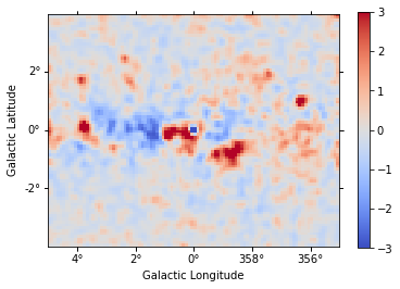
[37]:
residual = counts - dataset.npred()
residual.sum_over_axes().smooth("0.1 deg").plot(
    cmap="coolwarm", vmin=-3, vmax=3, add_cbar=True
);
Exercises#
Fit the position and spectrum of the source SNR G0.9+0.1.
Make maps and fit the position and spectrum of the Crab nebula.
Summary#
In this tutorial you have seen how to work with Fermi-LAT data with Gammapy. You have to use the Fermi ST to prepare the exposure cube and PSF, and then you can use Gammapy for any event or map analysis using the same methods that are used to analyse IACT data.
This works very well at high energies (here above 10 GeV), where the exposure and PSF is almost constant spatially and only varies a little with energy. It is not expected to give good results for low-energy data, where the Fermi-LAT PSF is very large. If you are interested to help us validate down to what energy Fermi-LAT analysis with Gammapy works well (e.g. by re-computing results from 3FHL or other published analysis results), or to extend the Gammapy capabilities (e.g. to work with energy-dependent multi-resolution maps and PSF), that would be very welcome!