This is a fixed-text formatted version of a Jupyter notebook

Try online
You may download all the notebooks as a tar file.
Source files: fitting.ipynb | fitting.py

Fitting#

Prerequisites#

Knowledge of spectral analysis to produce 1D On-Off datasets, see the following tutorial
Reading of pre-computed datasets see the MWL tutorial
General knowledge on statistics and optimization methods

Proposed approach#

This is a hands-on tutorial to gammapy.modeling, showing how to do perform a Fit in gammapy. The emphasis here is on interfacing the Fit class and inspecting the errors. To see an analysis example of how datasets and models interact, see the model management notebook. As an example, in this notebook, we are going to work with HESS data of the Crab Nebula and show in particular how to : - perform a spectral analysis - use different fitting backends - access covariance matrix information and parameter errors - compute likelihood profile - compute confidence contours

See also: Models gallery tutorial and docs/modeling/index.rst.

The setup#

[1]:

import numpy as np
from astropy import units as u
import matplotlib.pyplot as plt
from matplotlib.ticker import StrMethodFormatter
import scipy.stats as st
from gammapy.modeling import Fit
from gammapy.datasets import Datasets, SpectrumDatasetOnOff
from gammapy.modeling.models import LogParabolaSpectralModel, SkyModel
from gammapy.visualization.utils import plot_contour_line
from itertools import combinations

Model and dataset#

First we define the source model, here we need only a spectral model for which we choose a log-parabola

[2]:

crab_spectrum = LogParabolaSpectralModel(
    amplitude=1e-11 / u.cm**2 / u.s / u.TeV,
    reference=1 * u.TeV,
    alpha=2.3,
    beta=0.2,
)

crab_spectrum.alpha.max = 3
crab_spectrum.alpha.min = 1
crab_model = SkyModel(spectral_model=crab_spectrum, name="crab")

The data and background are read from pre-computed ON/OFF datasets of HESS observations, for simplicity we stack them together. Then we set the model and fit range to the resulting dataset.

[3]:

datasets = []
for obs_id in [23523, 23526]:
    dataset = SpectrumDatasetOnOff.read(
        f"$GAMMAPY_DATA/joint-crab/spectra/hess/pha_obs{obs_id}.fits"
    )
    datasets.append(dataset)

dataset_hess = Datasets(datasets).stack_reduce(name="HESS")
datasets = Datasets(datasets=[dataset_hess])

# Set model and fit range
dataset_hess.models = crab_model
e_min = 0.66 * u.TeV
e_max = 30 * u.TeV
dataset_hess.mask_fit = dataset_hess.counts.geom.energy_mask(e_min, e_max)

Fitting options#

First let’s create a Fit instance:

[4]:

scipy_opts = {
    "method": "L-BFGS-B",
    "options": {"ftol": 1e-4, "gtol": 1e-05},
    "backend": "scipy",
}
fit_scipy = Fit(store_trace=True, optimize_opts=scipy_opts)

By default the fit is performed using MINUIT, you can select alternative optimizers and set their option using the optimize_opts argument of the Fit.run() method. In addition we have specified to store the trace of parameter values of the fit.

Note that, for now, covaraince matrix and errors are computed only for the fitting with MINUIT. However depending on the problem other optimizers can better perform, so sometimes it can be useful to run a pre-fit with alternative optimization methods.

For the “scipy” backend the available options are described in detail here:

https://docs.scipy.org/doc/scipy/reference/generated/scipy.optimize.minimize.html

[5]:

%%time
result_scipy = fit_scipy.run(datasets)

CPU times: user 287 ms, sys: 5.44 ms, total: 292 ms
Wall time: 332 ms

For the “sherpa” backend you can choose the optimization algorithm between method = {“simplex”, “levmar”, “moncar”, “gridsearch”}.

Those methods are described and compared in detail on http://cxc.cfa.harvard.edu/sherpa/methods/index.html The available options of the optimization methods are described on the following page https://cxc.cfa.harvard.edu/sherpa/methods/opt_methods.html

[6]:

%%time
sherpa_opts = {"method": "simplex", "ftol": 1e-3, "maxfev": int(1e4)}
fit_sherpa = Fit(store_trace=True, backend="sherpa", optimize_opts=sherpa_opts)
results_simplex = fit_sherpa.run(datasets)

---------------------------------------------------------------------------
ModuleNotFoundError                       Traceback (most recent call last)
File <timed exec>:3, in <module>

File ~/github/adonath/gammapy/gammapy/modeling/fit.py:158, in Fit.run(self, datasets)
    145 def run(self, datasets):
    146     """Run all fitting steps.
    147
    148     Parameters
   (...)
    156         Fit result
    157     """
--> 158     optimize_result = self.optimize(datasets=datasets)
    160     if self.backend not in registry.register["covariance"]:
    161         log.warning("No covariance estimate - not supported by this backend.")

File ~/github/adonath/gammapy/gammapy/modeling/fit.py:196, in Fit.optimize(self, datasets)
    192 compute = registry.get("optimize", backend)
    193 # TODO: change this calling interface!
    194 # probably should pass a fit statistic, which has a model, which has parameters
    195 # and return something simpler, not a tuple of three things
--> 196 factors, info, optimizer = compute(
    197     parameters=parameters,
    198     function=datasets.stat_sum,
    199     store_trace=self.store_trace,
    200     **kwargs,
    201 )
    203 if backend == "minuit":
    204     self._minuit = optimizer

File ~/github/adonath/gammapy/gammapy/modeling/sherpa.py:50, in optimize_sherpa(parameters, function, store_trace, **kwargs)
     33 """Sherpa optimization wrapper method.
     34
     35 Parameters
   (...)
     47     Tuple containing the best fit factors, some info and the optimizer instance.
     48 """
     49 method = kwargs.pop("method", "simplex")
---> 50 optimizer = get_sherpa_optimizer(method)
     51 optimizer.config.update(kwargs)
     53 pars = [par.factor for par in parameters.free_parameters]

File ~/github/adonath/gammapy/gammapy/modeling/sherpa.py:9, in get_sherpa_optimizer(name)
      8 def get_sherpa_optimizer(name):
----> 9     from sherpa.optmethods import GridSearch, LevMar, MonCar, NelderMead
     11     return {
     12         "levmar": LevMar,
     13         "simplex": NelderMead,
     14         "moncar": MonCar,
     15         "gridsearch": GridSearch,
     16     }[name]()

ModuleNotFoundError: No module named 'sherpa'

For the “minuit” backend see https://iminuit.readthedocs.io/en/latest/reference.html for a detailed description of the available options. If there is an entry ‘migrad_opts’, those options will be passed to iminuit.Minuit.migrad. Additionally you can set the fit tolerance using the tol option. The minimization will stop when the estimated distance to the minimum is less than 0.001*tol (by default tol=0.1). The strategy option change the speed and accuracy of the optimizer: 0 fast, 1 default, 2 slow but accurate. If you want more reliable error estimates, you should run the final fit with strategy 2.

[7]:

%%time
fit = Fit(store_trace=True)
minuit_opts = {"tol": 0.001, "strategy": 1}
fit.backend = "minuit"
fit.optimize_opts = minuit_opts
result_minuit = fit.run(datasets)

CPU times: user 139 ms, sys: 3.12 ms, total: 142 ms
Wall time: 159 ms

Fit quality assessment#

There are various ways to check the convergence and quality of a fit. Among them:

Refer to the automatically-generated results dictionary:

[8]:

print(result_scipy)

OptimizeResult

        backend    : scipy
        method     : L-BFGS-B
        success    : True
        message    : CONVERGENCE: REL_REDUCTION_OF_F_<=_FACTR*EPSMCH
        nfev       : 60
        total stat : 30.35

CovarianceResult

        backend    : minuit
        method     : hesse
        success    : True
        message    : Hesse terminated successfully.

[9]:

print(results_simplex)

---------------------------------------------------------------------------
NameError                                 Traceback (most recent call last)
Input In [9], in <cell line: 1>()
----> 1 print(results_simplex)

NameError: name 'results_simplex' is not defined

[10]:

print(result_minuit)

OptimizeResult

        backend    : minuit
        method     : migrad
        success    : True
        message    : Optimization terminated successfully.
        nfev       : 52
        total stat : 30.35

CovarianceResult

        backend    : minuit
        method     : hesse
        success    : True
        message    : Hesse terminated successfully.

If the fit is performed with minuit you can print detailed informations to check the convergence

[11]:

print(fit.minuit)

┌─────────────────────────────────────────────────────────────────────────┐
│                                Migrad                                   │
├──────────────────────────────────┬──────────────────────────────────────┤
│ FCN = 30.35                      │              Nfcn = 52               │
│ EDM = 4.15e-10 (Goal: 2e-06)     │            time = 0.1 sec            │
├──────────────────────────────────┼──────────────────────────────────────┤
│          Valid Minimum           │        No Parameters at limit        │
├──────────────────────────────────┼──────────────────────────────────────┤
│ Below EDM threshold (goal x 10)  │           Below call limit           │
├───────────────┬──────────────────┼───────────┬─────────────┬────────────┤
│  Covariance   │     Hesse ok     │ Accurate  │  Pos. def.  │ Not forced │
└───────────────┴──────────────────┴───────────┴─────────────┴────────────┘
┌───┬───────────────────┬───────────┬───────────┬────────────┬────────────┬─────────┬─────────┬───────┐
│   │ Name              │   Value   │ Hesse Err │ Minos Err- │ Minos Err+ │ Limit-  │ Limit+  │ Fixed │
├───┼───────────────────┼───────────┼───────────┼────────────┼────────────┼─────────┼─────────┼───────┤
│ 0 │ par_000_amplitude │    3.8    │    0.4    │            │            │         │         │       │
│ 1 │ par_001_alpha     │   2.20    │   0.26    │            │            │    1    │    3    │       │
│ 2 │ par_002_beta      │    2.3    │    1.4    │            │            │         │         │       │
└───┴───────────────────┴───────────┴───────────┴────────────┴────────────┴─────────┴─────────┴───────┘
┌───────────────────┬───────────────────────────────────────────────────────┐
│                   │ par_000_amplitude     par_001_alpha      par_002_beta │
├───────────────────┼───────────────────────────────────────────────────────┤
│ par_000_amplitude │             0.126            0.0458            -0.119 │
│     par_001_alpha │            0.0458            0.0696            -0.335 │
│      par_002_beta │            -0.119            -0.335              1.97 │
└───────────────────┴───────────────────────────────────────────────────────┘

Check the trace of the fit e.g. in case the fit did not converge properly

[12]:

result_minuit.trace

[12]:

Table length=52

total_stat	crab.spectral.amplitude	crab.spectral.alpha	crab.spectral.beta
float64	float64	float64	float64
30.3500657162104	3.817289698656186e-11	2.197292407700903	0.22709127789012862
30.350283248175447	3.820841929575321e-11	2.197292407700903	0.22709127789012862
30.350222616485947	3.81373746773705e-11	2.197292407700903	0.22709127789012862
30.35007926860123	3.8179994706225424e-11	2.197292407700903	0.22709127789012862
30.350067112690233	3.816579926689829e-11	2.197292407700903	0.22709127789012862
30.352094318911043	3.817289698656186e-11	2.1999760722366375	0.22709127789012862
30.350029544745276	3.817289698656186e-11	2.19460726388853	0.22709127789012862
30.350179154484287	3.817289698656186e-11	2.1975608410540226	0.22709127789012862
30.349972202223313	3.817289698656186e-11	2.1970239595550076	0.22709127789012862
30.351857502861385	3.817289698656186e-11	2.197292407700903	0.22850114499290705
30.349837154420428	3.817289698656186e-11	2.197292407700903	0.2256814107873502
30.35017479159167	3.817289698656186e-11	2.197292407700903	0.22723226460040646
30.34997227296953	3.817289698656186e-11	2.197292407700903	0.2269502911798508
30.34997695393293	3.817001117496923e-11	2.1958980704229853	0.2261780173394799
30.34974235504521	3.8171338387753655e-11	2.1965393890554075	0.2265980347381994
30.349813792334285	3.817843607213018e-11	2.1965393890554075	0.2265980347381994
30.349685869600748	3.816424070337713e-11	2.1965393890554075	0.2265980347381994
30.349743320421467	3.8171338387753655e-11	2.1967719387411244	0.2265980347381994
30.349756399032348	3.8171338387753655e-11	2.1963068283133813	0.2265980347381994
30.349751959719185	3.8171338387753655e-11	2.1965393890554075	0.22673590512220493
30.349747780067773	3.8171338387753655e-11	2.1965393890554075	0.22646016435419383
30.349578125655736	3.8146127436317635e-11	2.1963598828820707	0.22641068578109103
30.349534163471766	3.8124657671199016e-11	2.196207009389486	0.2262511385258221
...	...	...	...
30.349534163471766	3.8124657671199016e-11	2.196207009389486	0.2262511385258221
30.349541897167885	3.8131754590818664e-11	2.196207009389486	0.2262511385258221
30.34954141331377	3.811756075157937e-11	2.196207009389486	0.2262511385258221
30.349543448344082	3.8124657671199016e-11	2.196439103828382	0.2262511385258221
30.34953983490288	3.8124657671199016e-11	2.1959749039576453	0.2262511385258221
30.349539830137537	3.8124657671199016e-11	2.196207009389486	0.22638863655365438
30.349543469018254	3.8124657671199016e-11	2.196207009389486	0.22611364049798982
30.34953451169259	3.8126077055122947e-11	2.196207009389486	0.2262511385258221
30.34953441459256	3.8123238287275085e-11	2.196207009389486	0.2262511385258221
30.349534824240266	3.8124657671199016e-11	2.1962534291571165	0.2262511385258221
30.34953410095561	3.8124657671199016e-11	2.196160589182137	0.2262511385258221
30.349534099466126	3.8124657671199016e-11	2.196207009389486	0.22627863813138857
30.34953482636601	3.8124657671199016e-11	2.196207009389486	0.22622363892025563
30.349541323317055	3.8131754590818664e-11	2.196439103828382	0.2262511385258221
30.349539387830283	3.8131754590818664e-11	2.196207009389486	0.22638863655365438
30.349563014685785	3.8124657671199016e-11	2.196439103828382	0.22638863655365438
30.349530433261027	3.812189947833074e-11	2.1957119982280755	0.22651087418268717
30.349537910866125	3.812898812391197e-11	2.1957119982280755	0.22651087418268717
30.349537906385564	3.81148108327495e-11	2.1957119982280755	0.22651087418268717
30.349537922340755	3.812189947833074e-11	2.195944056474383	0.22651087418268717
30.349537894602186	3.812189947833074e-11	2.195479929022191	0.22651087418268717
30.349537879388105	3.812189947833074e-11	2.1957119982280755	0.22664826384159636
30.349537929838906	3.812189947833074e-11	2.1957119982280755	0.22637348452377798

Check that the fitted values and errors for all parameters are reasonable, and no fitted parameter value is “too close” - or even outside - its allowed min-max range

[13]:

result_minuit.parameters.to_table()

[13]:

Table length=4

type	name	value	unit	error	min	max	frozen	is_norm	link
str8	str9	float64	str14	float64	float64	float64	bool	bool	str1
spectral	amplitude	3.8122e-11	cm-2 s-1 TeV-1	3.548e-12	nan	nan	False	True
spectral	reference	1.0000e+00	TeV	0.000e+00	nan	nan	True	False
spectral	alpha	2.1957e+00		2.639e-01	1.000e+00	3.000e+00	False	False
spectral	beta	2.2651e-01		1.403e-01	nan	nan	False	False

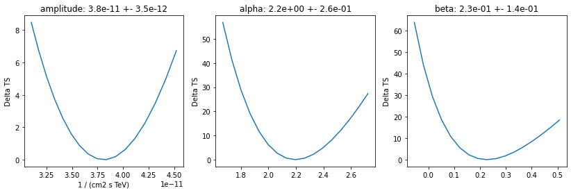
Plot fit statistic profiles for all fitted parameters, using gammapy.modeling.Fit.stat_profile(). For a good fit and error estimate each profile should be parabolic. The specification for each fit statistic profile can be changed on the gammapy.modeling.Parameter object, which has .scan_min, .scan_max, .scan_n_values and .scan_n_sigma attributes.

[14]:

total_stat = result_minuit.total_stat

fig, axes = plt.subplots(nrows=1, ncols=3, figsize=(14, 4))

for ax, par in zip(axes, crab_model.parameters.free_parameters):
    par.scan_n_values = 17

    profile = fit.stat_profile(datasets=datasets, parameter=par)
    ax.plot(profile[f"{par.name}_scan"], profile["stat_scan"] - total_stat)
    ax.set_xlabel(f"{par.unit}")
    ax.set_ylabel("Delta TS")
    ax.set_title(f"{par.name}: {par.value:.1e} +- {par.error:.1e}")

../../_images/tutorials_api_fitting_26_0.png

Inspect model residuals. Those can always be accessed using ~Dataset.residuals(), that will return an array in case a the fitted Dataset is a SpectrumDataset and a full cube in case of a MapDataset. For more details, we refer here to the dedicated fitting tutorials: analysis_3d.ipynb (for MapDataset fitting) and spectrum_analysis.ipynb (for SpectrumDataset fitting).

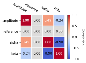
Covariance and parameters errors#

After the fit the covariance matrix is attached to the model. You can get the error on a specific parameter by accessing the .error attribute:

[15]:

crab_model.spectral_model.alpha.error

[15]:

0.26387706255272814

And you can plot the total parameter correlation as well:

[16]:

crab_model.covariance.plot_correlation()

[16]:

<AxesSubplot:>

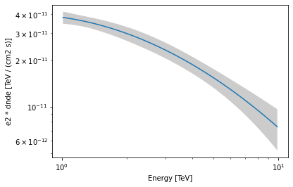
../../_images/tutorials_api_fitting_31_1.png

As an example, this step is needed to produce a butterfly plot showing the envelope of the model taking into account parameter uncertainties.

[17]:

energy_bounds = [1, 10] * u.TeV
crab_spectrum.plot(energy_bounds=energy_bounds, energy_power=2)
ax = crab_spectrum.plot_error(energy_bounds=energy_bounds, energy_power=2)

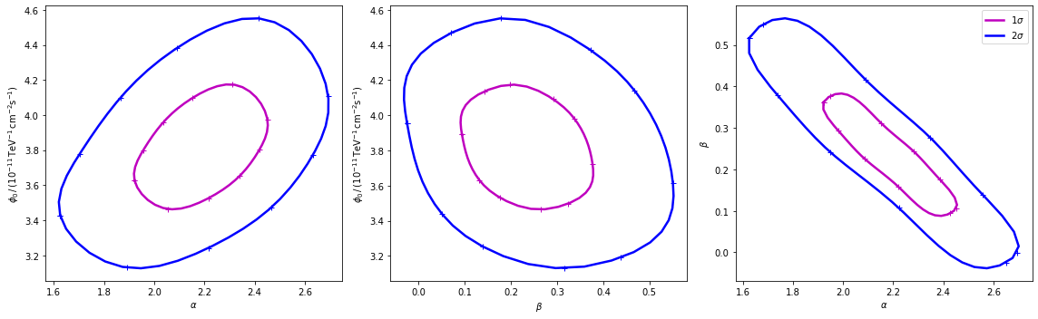
../../_images/tutorials_api_fitting_33_0.png

Confidence contours#

In most studies, one wishes to estimate parameters distribution using observed sample data. A 1-dimensional confidence interval gives an estimated range of values which is likely to include an unknown parameter. A confidence contour is a 2-dimensional generalization of a confidence interval, often represented as an ellipsoid around the best-fit value.

Gammapy offers two ways of computing confidence contours, in the dedicated methods Fit.minos_contour() and Fit.stat_profile(). In the following sections we will describe them.

An important point to keep in mind is: what does a :math:`Nsigma` confidence contour really mean? The answer is it represents the points of the parameter space for which the model likelihood is \(N\sigma\) above the minimum. But one always has to keep in mind that 1 standard deviation in two dimensions has a smaller coverage probability than 68%, and similarly for all other levels. In particular, in 2-dimensions the probability enclosed by the \(N\sigma\) confidence contour is \(P(N)=1-e^{-N^2/2}\).

Computing contours using `Fit.stat_contour()`#

After the fit, MINUIT offers the possibility to compute the confidence confours. gammapy provides an interface to this functionality through the Fit object using the .stat_contour method. Here we defined a function to automate the contour production for the different parameterer and confidence levels (expressed in term of sigma):

[18]:

def make_contours(fit, datasets, result, npoints, sigmas):
    cts_sigma = []
    for sigma in sigmas:
        contours = dict()
        for par_1, par_2 in combinations(["alpha", "beta", "amplitude"], r=2):
            contour = fit.stat_contour(
                datasets=datasets,
                x=datasets.parameters[par_1],
                y=datasets.parameters[par_2],
                numpoints=npoints,
                sigma=sigma,
            )
            contours[f"contour_{par_1}_{par_2}"] = {
                par_1: contour[par_1].tolist(),
                par_2: contour[par_2].tolist(),
            }
        cts_sigma.append(contours)
    return cts_sigma

Now we can compute few contours.

[19]:

%%time
sigmas = [1, 2]
cts_sigma = make_contours(
    fit=fit,
    datasets=datasets,
    result=result_minuit,
    npoints=10,
    sigmas=sigmas,
)

/Users/adonath/software/mambaforge/envs/gammapy-dev/lib/python3.9/site-packages/numpy/core/fromnumeric.py:86: RuntimeWarning: overflow encountered in reduce
  return ufunc.reduce(obj, axis, dtype, out, **passkwargs)

CPU times: user 10.5 s, sys: 130 ms, total: 10.6 s
Wall time: 13 s

Then we prepare some aliases and annotations in order to make the plotting nicer.

[20]:

pars = {
    "phi": r"$\phi_0 \,/\,(10^{-11}\,{\rm TeV}^{-1} \, {\rm cm}^{-2} {\rm s}^{-1})$",
    "alpha": r"$\alpha$",
    "beta": r"$\beta$",
}

panels = [
    {
        "x": "alpha",
        "y": "phi",
        "cx": (lambda ct: ct["contour_alpha_amplitude"]["alpha"]),
        "cy": (
            lambda ct: np.array(1e11)
            * ct["contour_alpha_amplitude"]["amplitude"]
        ),
    },
    {
        "x": "beta",
        "y": "phi",
        "cx": (lambda ct: ct["contour_beta_amplitude"]["beta"]),
        "cy": (
            lambda ct: np.array(1e11)
            * ct["contour_beta_amplitude"]["amplitude"]
        ),
    },
    {
        "x": "alpha",
        "y": "beta",
        "cx": (lambda ct: ct["contour_alpha_beta"]["alpha"]),
        "cy": (lambda ct: ct["contour_alpha_beta"]["beta"]),
    },
]

Finally we produce the confidence contours figures.

[21]:

fig, axes = plt.subplots(1, 3, figsize=(16, 5))
colors = ["m", "b", "c"]
for p, ax in zip(panels, axes):
    xlabel = pars[p["x"]]
    ylabel = pars[p["y"]]
    for ks in range(len(cts_sigma)):
        plot_contour_line(
            ax,
            p["cx"](cts_sigma[ks]),
            p["cy"](cts_sigma[ks]),
            lw=2.5,
            color=colors[ks],
            label=f"{sigmas[ks]}" + r"$\sigma$",
        )
    ax.set_xlabel(xlabel)
    ax.set_ylabel(ylabel)
plt.legend()
plt.tight_layout()

../../_images/tutorials_api_fitting_44_0.png

Computing contours using `Fit.stat_surface()`#

This alternative method for the computation of confidence contours, although more time consuming than Fit.minos_contour(), is expected to be more stable. It consists of a generalization of Fit.stat_profile() to a 2-dimensional parameter space. The algorithm is very simple: - First, passing two arrays of parameters values, a 2-dimensional discrete parameter space is defined; - For each node of the parameter space, the two parameters of interest are frozen. This way, a likelihood value (\(-2\mathrm{ln}\,\mathcal{L}\), actually) is computed, by either freezing (default) or fitting all nuisance parameters; - Finally, a 2-dimensional surface of \(-2\mathrm{ln}(\mathcal{L})\) values is returned. Using that surface, one can easily compute a surface of \(TS = -2\Delta\mathrm{ln}(\mathcal{L})\) and compute confidence contours.

Let’s see it step by step.

First of all, we can notice that this method is “backend-agnostic”, meaning that it can be run with MINUIT, sherpa or scipy as fitting tools. Here we will stick with MINUIT, which is the default choice:

[ ]:

As an example, we can compute the confidence contour for the alpha and beta parameters of the dataset_hess. Here we define the parameter space:

[22]:

result = result_minuit
par_alpha = datasets.parameters["alpha"]
par_beta = datasets.parameters["beta"]

par_alpha.scan_values = np.linspace(1.55, 2.7, 20)
par_beta.scan_values = np.linspace(-0.05, 0.55, 20)

Then we run the algorithm, by choosing reoptimize=False for the sake of time saving. In real life applications, we strongly recommend to use reoptimize=True, so that all free nuisance parameters will be fit at each grid node. This is the correct way, statistically speaking, of computing confidence contours, but is expected to be time consuming.

[23]:

fit = Fit(backend="minuit", optimize_opts={"print_level": 0})
stat_surface = fit.stat_surface(
    datasets=datasets,
    x=par_alpha,
    y=par_beta,
    reoptimize=False,
)

In order to easily inspect the results, we can convert the \(-2\mathrm{ln}(\mathcal{L})\) surface to a surface of statistical significance (in units of Gaussian standard deviations from the surface minimum):

[24]:

# Compute TS
TS = stat_surface["stat_scan"] - result.total_stat

[25]:

# Compute the corresponding statistical significance surface
stat_surface = np.sqrt(TS.T)

Notice that, as explained before, \(1\sigma\) contour obtained this way will not contain 68% of the probability, but rather

[26]:

# Compute the corresponding statistical significance surface
# p_value = 1 - st.chi2(df=1).cdf(TS)
# gaussian_sigmas = st.norm.isf(p_value / 2).T

Finally, we can plot the surface values together with contours:

[27]:

fig, ax = plt.subplots(figsize=(8, 6))
x_values = par_alpha.scan_values
y_values = par_beta.scan_values

# plot surface
im = ax.pcolormesh(x_values, y_values, stat_surface, shading="auto")
fig.colorbar(im, label="sqrt(TS)")
ax.set_xlabel(f"{par_alpha.name}")
ax.set_ylabel(f"{par_beta.name}")

# We choose to plot 1 and 2 sigma confidence contours
levels = [1, 2]
contours = ax.contour(
    x_values, y_values, stat_surface, levels=levels, colors="white"
)
ax.clabel(contours, fmt="%.0f$\,\sigma$", inline=3, fontsize=15);

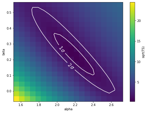
../../_images/tutorials_api_fitting_59_0.png

Note that, if computed with reoptimize=True, this plot would be completely consistent with the third panel of the plot produced with Fit.stat_contour (try!).

Finally, it is always remember that confidence contours are approximations. In particular, when the parameter range boundaries are close to the contours lines, it is expected that the statistical meaning of the contours is not well defined. That’s why we advise to always choose a parameter space that com contain the contours you’re interested in.

[ ]: