Note
Click here to download the full example code or to run this example in your browser via Binder
Ring background map#
Create an excess (gamma-ray events) and a significance map extracting a ring background.
Context#
One of the challenges of IACT analysis is accounting for the large residual hadronic emission. An excess map, assumed to be a map of only gamma-ray events, requires a good estimate of the background. However, in the absence of a solid template bkg model it is not possible to obtain reliable background model a priori. It was often found necessary in classical cherenkov astronomy to perform a local renormalization of the existing templates, usually with a ring kernel. This assumes that most of the events are background and requires to have an exclusion mask to remove regions with bright signal from the estimation. To read more about this method, see here.
Objective#
Create an excess (gamma-ray events) map of MSH 15-52 as well as a significance map to determine how solid the signal is.
Proposed approach#
The analysis workflow is roughly:
Compute the sky maps keeping each observation separately using the
AnalysisclassEstimate the background using the
RingBackgroundMakerCompute the correlated excess and significance maps using the
ExcessMapEstimator
The normalised background thus obtained can be used for general modelling and fitting.
Setup#
As usual, we’ll start with some general imports…
import logging
import numpy as np
from scipy.stats import norm

# %matplotlib inline
import astropy.units as u
from astropy.coordinates import SkyCoord
from regions import CircleSkyRegion
import matplotlib.pyplot as plt
from gammapy.analysis import Analysis, AnalysisConfig
from gammapy.datasets import MapDatasetOnOff
from gammapy.estimators import ExcessMapEstimator
from gammapy.makers import RingBackgroundMaker

log = logging.getLogger(__name__)
Check setup#
from gammapy.utils.check import check_tutorials_setup

check_tutorials_setup()
System:

        python_executable      : /home/runner/work/gammapy-docs/gammapy-docs/gammapy/.tox/build_docs/bin/python
        python_version         : 3.9.15
        machine                : x86_64
        system                 : Linux


Gammapy package:

        version                : 1.0
        path                   : /home/runner/work/gammapy-docs/gammapy-docs/gammapy/.tox/build_docs/lib/python3.9/site-packages/gammapy


Other packages:

        numpy                  : 1.23.4
        scipy                  : 1.9.3
        astropy                : 5.1.1
        regions                : 0.7
        click                  : 8.1.3
        yaml                   : 6.0
        IPython                : 8.6.0
        jupyterlab             : not installed
        matplotlib             : 3.6.2
        pandas                 : not installed
        healpy                 : 1.16.1
        iminuit                : 2.17.0
        sherpa                 : 4.15.0
        naima                  : 0.10.0
        emcee                  : 3.1.3
        corner                 : 2.2.1


Gammapy environment variables:

        GAMMAPY_DATA           : /home/runner/work/gammapy-docs/gammapy-docs/gammapy-datasets/1.0
Creating the config file#
Now, we create a config file for out analysis. You may load this from disc if you have a pre-defined config file.
In this example, we will use a few HESS runs on the pulsar wind nebula, MSH 1552
# source_pos = SkyCoord.from_name("MSH 15-52")
source_pos = SkyCoord(228.32, -59.08, unit="deg")

config = AnalysisConfig()
# Select observations - 2.5 degrees from the source position
config.observations.datastore = "$GAMMAPY_DATA/hess-dl3-dr1/"
config.observations.obs_cone = {
    "frame": "icrs",
    "lon": source_pos.ra,
    "lat": source_pos.dec,
    "radius": 2.5 * u.deg,
}

config.datasets.type = "3d"
config.datasets.geom.wcs.skydir = {
    "lon": source_pos.ra,
    "lat": source_pos.dec,
    "frame": "icrs",
}  # The WCS geometry - centered on MSH 15-52
config.datasets.geom.wcs.width = {"width": "3 deg", "height": "3 deg"}
config.datasets.geom.wcs.binsize = "0.02 deg"

# Cutout size (for the run-wise event selection)
config.datasets.geom.selection.offset_max = 3.5 * u.deg

# We now fix the energy axis for the counts map - (the reconstructed energy binning)
config.datasets.geom.axes.energy.min = "0.5 TeV"
config.datasets.geom.axes.energy.max = "5 TeV"
config.datasets.geom.axes.energy.nbins = 10

# We need to extract the ring for each observation separately, hence, no stacking at this stage
config.datasets.stack = False

print(config)
AnalysisConfig

    general:
        log: {level: info, filename: null, filemode: null, format: null, datefmt: null}
        outdir: .
        n_jobs: 1
        datasets_file: null
        models_file: null
    observations:
        datastore: $GAMMAPY_DATA/hess-dl3-dr1
        obs_ids: []
        obs_file: null
        obs_cone: {frame: icrs, lon: 228.32 deg, lat: -59.08 deg, radius: 2.5 deg}
        obs_time: {start: null, stop: null}
        required_irf: [aeff, edisp, psf, bkg]
    datasets:
        type: 3d
        stack: false
        geom:
            wcs:
                skydir: {frame: icrs, lon: 228.32 deg, lat: -59.08 deg}
                binsize: 0.02 deg
                width: {width: 3.0 deg, height: 3.0 deg}
                binsize_irf: 0.2 deg
            selection: {offset_max: 3.5 deg}
            axes:
                energy: {min: 0.5 TeV, max: 5.0 TeV, nbins: 10}
                energy_true: {min: 0.5 TeV, max: 20.0 TeV, nbins: 16}
        map_selection: [counts, exposure, background, psf, edisp]
        background:
            method: null
            exclusion: null
            parameters: {}
        safe_mask:
            methods: [aeff-default]
            parameters: {}
        on_region: {frame: null, lon: null, lat: null, radius: null}
        containment_correction: true
    fit:
        fit_range: {min: null, max: null}
    flux_points:
        energy: {min: null, max: null, nbins: null}
        source: source
        parameters: {selection_optional: all}
    excess_map:
        correlation_radius: 0.1 deg
        parameters: {}
        energy_edges: {min: null, max: null, nbins: null}
    light_curve:
        time_intervals: {start: null, stop: null}
        energy_edges: {min: null, max: null, nbins: null}
        source: source
        parameters: {selection_optional: all}
Getting the reduced dataset#
We now use the config file to do the initial data reduction which will then be used for a ring extraction
create the config
analysis = Analysis(config)

# for this specific case,w e do not need fine bins in true energy
analysis.config.datasets.geom.axes.energy_true = (
    analysis.config.datasets.geom.axes.energy
)

# `First get the required observations
analysis.get_observations()

print(analysis.config)
AnalysisConfig

    general:
        log: {level: INFO, filename: null, filemode: null, format: null, datefmt: null}
        outdir: .
        n_jobs: 1
        datasets_file: null
        models_file: null
    observations:
        datastore: $GAMMAPY_DATA/hess-dl3-dr1
        obs_ids: []
        obs_file: null
        obs_cone: {frame: icrs, lon: 228.32 deg, lat: -59.08 deg, radius: 2.5 deg}
        obs_time: {start: null, stop: null}
        required_irf: [aeff, edisp, psf, bkg]
    datasets:
        type: 3d
        stack: false
        geom:
            wcs:
                skydir: {frame: icrs, lon: 228.32 deg, lat: -59.08 deg}
                binsize: 0.02 deg
                width: {width: 3.0 deg, height: 3.0 deg}
                binsize_irf: 0.2 deg
            selection: {offset_max: 3.5 deg}
            axes:
                energy: {min: 0.5 TeV, max: 5.0 TeV, nbins: 10}
                energy_true: {min: 0.5 TeV, max: 5.0 TeV, nbins: 10}
        map_selection: [counts, exposure, background, psf, edisp]
        background:
            method: null
            exclusion: null
            parameters: {}
        safe_mask:
            methods: [aeff-default]
            parameters: {}
        on_region: {frame: null, lon: null, lat: null, radius: null}
        containment_correction: true
    fit:
        fit_range: {min: null, max: null}
    flux_points:
        energy: {min: null, max: null, nbins: null}
        source: source
        parameters: {selection_optional: all}
    excess_map:
        correlation_radius: 0.1 deg
        parameters: {}
        energy_edges: {min: null, max: null, nbins: null}
    light_curve:
        time_intervals: {start: null, stop: null}
        energy_edges: {min: null, max: null, nbins: null}
        source: source
        parameters: {selection_optional: all}
Data extraction
Extracting the ring background#
Since the ring background is extracted from real off events, we need to
use the wstat statistics in this case. For this, we will use the
MapDatasetOnOFF and the RingBackgroundMaker classes.
Create exclusion mask#
First, we need to create an exclusion mask on the known sources. In this
case, we need to mask only MSH 15-52 but this depends on the sources
present in our field of view.
# get the geom that we use
geom = analysis.datasets[0].counts.geom
energy_axis = analysis.datasets[0].counts.geom.axes["energy"]
geom_image = geom.to_image().to_cube([energy_axis.squash()])

# Make the exclusion mask
regions = CircleSkyRegion(center=source_pos, radius=0.3 * u.deg)
exclusion_mask = ~geom_image.region_mask([regions])
exclusion_mask.sum_over_axes().plot()
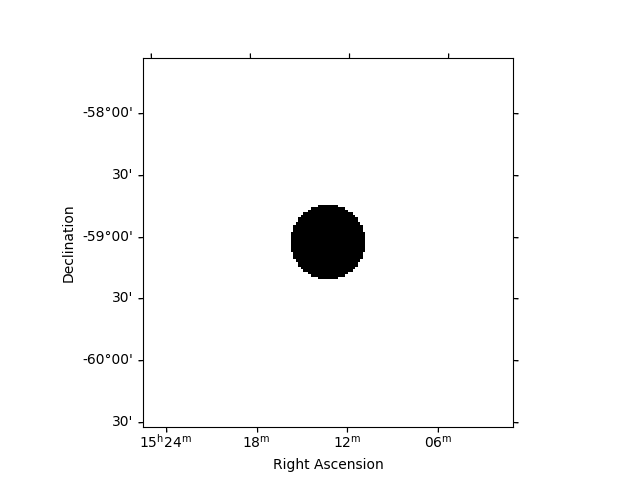
<WCSAxesSubplot: >
For the present analysis, we use a ring with an inner radius of 0.5 deg and width of 0.3 deg.
ring_maker = RingBackgroundMaker(
    r_in="0.5 deg", width="0.3 deg", exclusion_mask=exclusion_mask
)
Create a stacked dataset#
Now, we extract the background for each dataset and then stack the maps together to create a single stacked map for further analysis
energy_axis_true = analysis.datasets[0].exposure.geom.axes["energy_true"]
stacked_on_off = MapDatasetOnOff.create(
    geom=geom_image, energy_axis_true=energy_axis_true, name="stacked"
)

for dataset in analysis.datasets:
    # Ring extracting makes sense only for 2D analysis
    dataset_on_off = ring_maker.run(dataset.to_image())
    stacked_on_off.stack(dataset_on_off)
This stacked_on_off has on and off counts and acceptance
maps which we will use in all further analysis. The acceptance and
acceptance_off maps are the system acceptance of gamma-ray like
events in the on and off regions respectively.
print(stacked_on_off)
MapDatasetOnOff
---------------

  Name                            : stacked

  Total counts                    : 40051
  Total background counts         : 39151.26
  Total excess counts             : 899.74

  Predicted counts                : 39151.62
  Predicted background counts     : 39151.62
  Predicted excess counts         : nan

  Exposure min                    : 1.11e+09 m2 s
  Exposure max                    : 1.30e+10 m2 s

  Number of total bins            : 22500
  Number of fit bins              : 22500

  Fit statistic type              : wstat
  Fit statistic value (-2 log(L)) : 26392.57

  Number of models                : 0
  Number of parameters            : 0
  Number of free parameters       : 0

  Total counts_off                : 88113384
  Acceptance                      : 22500
  Acceptance off                  : 49447600
Compute correlated significance and correlated excess maps#
We need to convolve our maps with an appropriate smoothing kernel. The significance is computed according to the Li & Ma expression for ON and OFF Poisson measurements, see here. Since astropy convolution kernels only accept integers, we first convert our required size in degrees to int depending on our pixel size.
# Using a convolution radius of 0.04 degrees
estimator = ExcessMapEstimator(0.04 * u.deg, selection_optional=[])
lima_maps = estimator.run(stacked_on_off)

significance_map = lima_maps["sqrt_ts"]
excess_map = lima_maps["npred_excess"]

# We can plot the excess and significance maps
fig, (ax1, ax2) = plt.subplots(
    figsize=(11, 5), subplot_kw={"projection": lima_maps.geom.wcs}, ncols=2
)

ax1.set_title("Significance map")
significance_map.plot(ax=ax1, add_cbar=True)

ax2.set_title("Excess map")
excess_map.plot(ax=ax2, add_cbar=True)
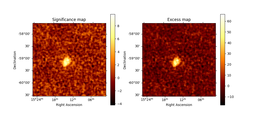
<WCSAxesSubplot: title={'center': 'Excess map'}>
It is often important to look at the signficance distribution outside the exclusion region to check that the background estimation is not contaminated by gamma-ray events. This can be the case when exclusion regions are not large enough. Typically, we expect the off distribution to be a standard normal distribution.
# create a 2D mask for the images
significance_map_off = significance_map * exclusion_mask
significance_all = significance_map.data[np.isfinite(significance_map.data)]
significance_off = significance_map_off.data[np.isfinite(significance_map_off.data)]

fig, ax = plt.subplots()
ax.hist(
    significance_all,
    density=True,
    alpha=0.5,
    color="red",
    label="all bins",
    bins=21,
)

ax.hist(
    significance_off,
    density=True,
    alpha=0.5,
    color="blue",
    label="off bins",
    bins=21,
)

# Now, fit the off distribution with a Gaussian
mu, std = norm.fit(significance_off)
x = np.linspace(-8, 8, 50)
p = norm.pdf(x, mu, std)
ax.plot(x, p, lw=2, color="black")
ax.legend()
ax.set_xlabel("Significance")
ax.set_yscale("log")
ax.set_ylim(1e-5, 1)
xmin, xmax = np.min(significance_all), np.max(significance_all)
ax.set_xlim(xmin, xmax)

print(f"Fit results: mu = {mu:.2f}, std = {std:.2f}")
plt.show()

# sphinx_gallery_thumbnail_number = 2
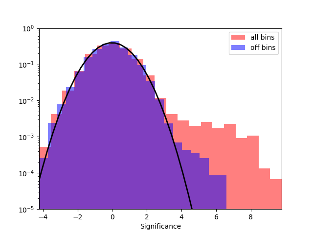
Fit results: mu = -0.02, std = 1.00
Total running time of the script: ( 0 minutes 18.881 seconds)