Light curves

Compute per-observation and nightly fluxes of four Crab nebula observations.

Prerequisites

• Knowledge of the high level interface to perform data reduction, see High level interface tutorial.

Context

This tutorial presents how light curve extraction is performed in gammapy, i.e. how to measure the flux of a source in different time bins.

Cherenkov telescopes usually work with observing runs and distribute data according to this basic time interval. A typical use case is to look for variability of a source on various time binnings: observation run-wise binning, nightly, weekly etc.

Objective: The Crab nebula is not known to be variable at TeV energies, so we expect constant brightness within statistical and systematic errors. Compute per-observation and nightly fluxes of the four Crab nebula observations from the H.E.S.S. first public test data releaseoto check it.

Proposed approach

We will demonstrate how to compute a light curve from 3D reduced datasets (MapDataset) as well as 1D ON-OFF spectral datasets (SpectrumDatasetOnOff).

The data reduction will be performed with the high level interface for the data reduction. Then we will use the LightCurveEstimator class, which is able to extract a light curve independently of the dataset type.

Setup

As usual, we’ll start with some general imports…

import logging
import astropy.units as u
from astropy.coordinates import SkyCoord
from astropy.time import Time

# %matplotlib inline
import matplotlib.pyplot as plt
from IPython.display import display
from gammapy.analysis import Analysis, AnalysisConfig
from gammapy.estimators import LightCurveEstimator
from gammapy.modeling.models import (
    Models,
    PointSpatialModel,
    PowerLawSpectralModel,
    SkyModel,
)

log = logging.getLogger(__name__)

Check setup

from gammapy.utils.check import check_tutorials_setup

check_tutorials_setup()

System:

        python_executable      : /home/runner/work/gammapy-docs/gammapy-docs/gammapy/.tox/build_docs/bin/python
        python_version         : 3.9.15
        machine                : x86_64
        system                 : Linux


Gammapy package:

        version                : 1.0
        path                   : /home/runner/work/gammapy-docs/gammapy-docs/gammapy/.tox/build_docs/lib/python3.9/site-packages/gammapy


Other packages:

        numpy                  : 1.23.4
        scipy                  : 1.9.3
        astropy                : 5.1.1
        regions                : 0.7
        click                  : 8.1.3
        yaml                   : 6.0
        IPython                : 8.6.0
        jupyterlab             : not installed
        matplotlib             : 3.6.2
        pandas                 : not installed
        healpy                 : 1.16.1
        iminuit                : 2.17.0
        sherpa                 : 4.15.0
        naima                  : 0.10.0
        emcee                  : 3.1.3
        corner                 : 2.2.1


Gammapy environment variables:

        GAMMAPY_DATA           : /home/runner/work/gammapy-docs/gammapy-docs/gammapy-datasets/1.0

Analysis configuration

For the 1D and 3D extraction, we will use the same CrabNebula configuration than in the High level interface tutorial using the high level interface of Gammapy.

From the high level interface, the data reduction for those observations is performed as followed

Building the 3D analysis configuration

conf_3d = AnalysisConfig()

Definition of the data selection

Here we use the Crab runs from the HESS DL3 data release 1

conf_3d.observations.obs_ids = [23523, 23526, 23559, 23592]

Definition of the dataset geometry

# We want a 3D analysis
conf_3d.datasets.type = "3d"

# We want to extract the data by observation and therefore to not stack them
conf_3d.datasets.stack = False

# Here is the WCS geometry of the Maps
conf_3d.datasets.geom.wcs.skydir = dict(
    frame="icrs", lon=83.63308 * u.deg, lat=22.01450 * u.deg
)
conf_3d.datasets.geom.wcs.binsize = 0.02 * u.deg
conf_3d.datasets.geom.wcs.width = dict(width=1 * u.deg, height=1 * u.deg)

# We define a value for the IRF Maps binsize
conf_3d.datasets.geom.wcs.binsize_irf = 0.2 * u.deg

# Define energy binning for the Maps
conf_3d.datasets.geom.axes.energy = dict(min=0.7 * u.TeV, max=10 * u.TeV, nbins=5)
conf_3d.datasets.geom.axes.energy_true = dict(min=0.3 * u.TeV, max=20 * u.TeV, nbins=20)

Run the 3D data reduction

analysis_3d = Analysis(conf_3d)
analysis_3d.get_observations()
analysis_3d.get_datasets()

Define the model to be used

Here we don’t try to fit the model parameters to the whole dataset, but we use predefined values instead.

target_position = SkyCoord(ra=83.63308, dec=22.01450, unit="deg")
spatial_model = PointSpatialModel(
    lon_0=target_position.ra, lat_0=target_position.dec, frame="icrs"
)

spectral_model = PowerLawSpectralModel(
    index=2.702,
    amplitude=4.712e-11 * u.Unit("1 / (cm2 s TeV)"),
    reference=1 * u.TeV,
)

sky_model = SkyModel(
    spatial_model=spatial_model, spectral_model=spectral_model, name="crab"
)

We assign them the model to be fitted to each dataset

models = Models([sky_model])
analysis_3d.set_models(models)

Light Curve estimation by observation

We can now create the light curve estimator.

We pass it the list of datasets and the name of the model component for which we want to build the light curve. In a given time bin, the only free parameter of the source is its normalization. We can optionally ask for parameters of other model components to be reoptimized during fit, that is most of the time to fit background normalization in each time bin.

If we don’t set any time interval, the LightCurveEstimator is determines the flux of each dataset and places it at the corresponding time in the light curve. Here one dataset equals to one observing run.

lc_maker_3d = LightCurveEstimator(
    energy_edges=[1, 10] * u.TeV, source="crab", reoptimize=False
)
# Example showing how to change some parameters from the object itself
lc_maker_3d.n_sigma_ul = 3  # Number of sigma to use for upper limit computation
lc_maker_3d.selection_optional = (
    "all"  # Add the computation of upper limits and likelihood profile
)
lc_3d = lc_maker_3d.run(analysis_3d.datasets)

The LightCurve object contains a table which we can explore.

# Example showing how to change just before plotting the threshold on the signal significance
# (points vs upper limits), even if this has no effect with this data set.
fig, ax = plt.subplots(
    figsize=(8, 6),
    gridspec_kw={"left": 0.16, "bottom": 0.2, "top": 0.98, "right": 0.98},
)
lc_3d.sqrt_ts_threshold_ul = 5
lc_3d.plot(ax=ax, axis_name="time")

table = lc_3d.to_table(format="lightcurve", sed_type="flux")
display(table["time_min", "time_max", "e_min", "e_max", "flux", "flux_err"])

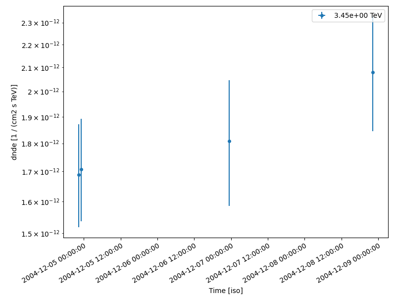
     time_min           time_max      ...        flux_err
                                      ...      1 / (cm2 s)
------------------ ------------------ ... ----------------------
53343.922340092584  53343.94186555555 ... 2.1205834122658536e-12
53343.954215092584  53343.97369425925 ... 2.1406685758704787e-12
 53345.96198129629  53345.98149518518 ...  2.789371501900168e-12
 53347.91319657407 53347.932710462956 ... 2.9141724875797992e-12

Running the light curve extraction in 1D

Building the 1D analysis configuration

conf_1d = AnalysisConfig()

Definition of the data selection

Here we use the Crab runs from the HESS DL3 data release 1

conf_1d.observations.obs_ids = [23523, 23526, 23559, 23592]

Definition of the dataset geometry

# We want a 1D analysis
conf_1d.datasets.type = "1d"

# We want to extract the data by observation and therefore to not stack them
conf_1d.datasets.stack = False

# Here we define the ON region and make sure that PSF leakage is corrected
conf_1d.datasets.on_region = dict(
    frame="icrs",
    lon=83.63308 * u.deg,
    lat=22.01450 * u.deg,
    radius=0.1 * u.deg,
)
conf_1d.datasets.containment_correction = True

# Finally we define the energy binning for the spectra
conf_1d.datasets.geom.axes.energy = dict(min=0.7 * u.TeV, max=10 * u.TeV, nbins=5)
conf_1d.datasets.geom.axes.energy_true = dict(min=0.3 * u.TeV, max=20 * u.TeV, nbins=20)

Run the 1D data reduction

analysis_1d = Analysis(conf_1d)
analysis_1d.get_observations()
analysis_1d.get_datasets()

Define the model to be used

Here we don’t try to fit the model parameters to the whole dataset, but we use predefined values instead.

target_position = SkyCoord(ra=83.63308, dec=22.01450, unit="deg")

spectral_model = PowerLawSpectralModel(
    index=2.702,
    amplitude=4.712e-11 * u.Unit("1 / (cm2 s TeV)"),
    reference=1 * u.TeV,
)

sky_model = SkyModel(spectral_model=spectral_model, name="crab")

We assign the model to be fitted to each dataset. We can use the same SkyModel as before.

models = Models([sky_model])
analysis_1d.set_models(models)

Extracting the light curve

lc_maker_1d = LightCurveEstimator(
    energy_edges=[1, 10] * u.TeV, source="crab", reoptimize=False
)
lc_1d = lc_maker_1d.run(analysis_1d.datasets)

print(lc_1d.geom.axes.names)

display(lc_1d.to_table(sed_type="flux", format="lightcurve"))

['energy', 'time']
     time_min           time_max            e_ref        ...    counts   success
                                             TeV         ...
------------------ ------------------ ------------------ ... ----------- -------
53343.922340092584  53343.94186555555 3.4517490659800814 ...  nan .. nan    True
53343.954215092584  53343.97369425925 3.4517490659800814 ... 71.0 .. nan    True
 53345.96198129629  53345.98149518518 3.4517490659800814 ...  nan .. nan    True
 53347.91319657407 53347.932710462956 3.4517490659800814 ... nan .. 59.0    True

Compare results

Finally we compare the result for the 1D and 3D lightcurve in a single figure:

fig, ax = plt.subplots(
    figsize=(8, 6),
    gridspec_kw={"left": 0.16, "bottom": 0.2, "top": 0.98, "right": 0.98},
)
lc_1d.plot(ax=ax, marker="o", label="1D")
lc_3d.plot(ax=ax, marker="o", label="3D")
plt.legend()

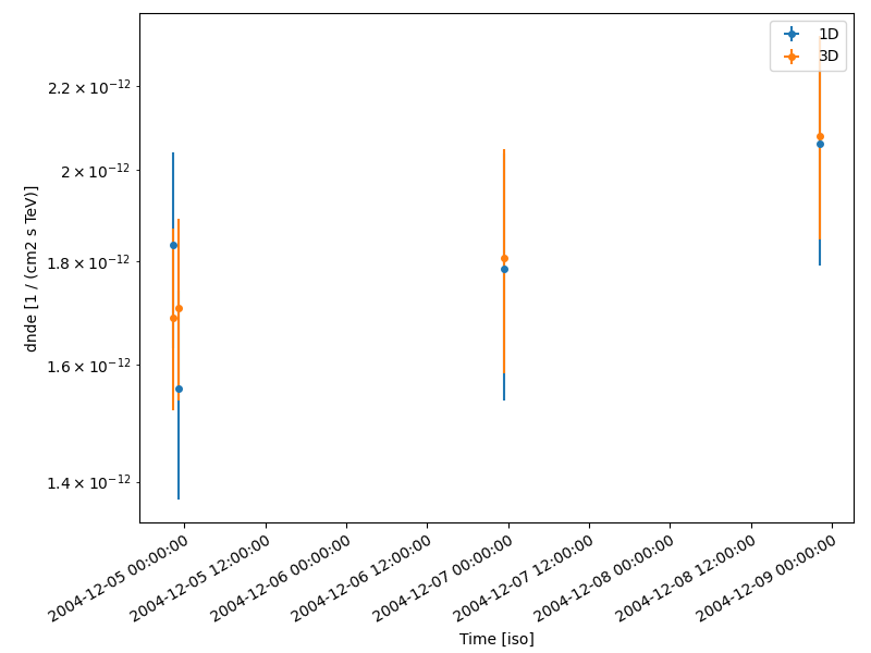
<matplotlib.legend.Legend object at 0x7f8330161b80>

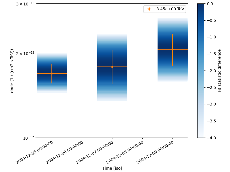
Night-wise LC estimation

Here we want to extract a night curve per night. We define the time intervals that cover the three nights.

time_intervals = [
    Time([53343.5, 53344.5], format="mjd", scale="utc"),
    Time([53345.5, 53346.5], format="mjd", scale="utc"),
    Time([53347.5, 53348.5], format="mjd", scale="utc"),
]

To compute the LC on the time intervals defined above, we pass the LightCurveEstimator the list of time intervals.

Internally, datasets are grouped per time interval and a flux extraction is performed for each group.

lc_maker_1d = LightCurveEstimator(
    energy_edges=[1, 10] * u.TeV,
    time_intervals=time_intervals,
    source="crab",
    reoptimize=False,
    selection_optional="all",
)

nightwise_lc = lc_maker_1d.run(analysis_1d.datasets)

fig, ax = plt.subplots(
    figsize=(8, 6),
    gridspec_kw={"left": 0.16, "bottom": 0.2, "top": 0.98, "right": 0.98},
)
nightwise_lc.plot(ax=ax, color="tab:orange")
nightwise_lc.plot_ts_profiles(ax=ax)
ax.set_ylim(1e-12, 3e-12)

plt.show()

What next?

When sources are bright enough to look for variability at small time scales, the per-observation time binning is no longer relevant. One can easily extend the light curve estimation approach presented above to any time binning. This is demonstrated in the Light curves for flares tutorial. which shows the extraction of the lightcurve of an AGN flare.