Note
Click here to download the full example code or to run this example in your browser via Binder
Point source sensitivity#
Estimate the CTA sensitivity for a point-like IRF at a fixed zenith angle and fixed offset.
Introduction#
This notebook explains how to estimate the CTA sensitivity for a point-like IRF at a fixed zenith angle and fixed offset using the full containment IRFs distributed for the CTA 1DC. The significance is computed for a 1D analysis (On-OFF regions) and the LiMa formula.
We use here an approximate approach with an energy dependent integration radius to take into account the variation of the PSF. We will first determine the 1D IRFs including a containment correction.
We will be using the following Gammapy class:
import numpy as np
import astropy.units as u
from astropy.coordinates import SkyCoord

# %matplotlib inline
import matplotlib.pyplot as plt
Setup#
As usual, we’ll start with some setup …
from IPython.display import display
from gammapy.data import Observation, observatory_locations
from gammapy.datasets import SpectrumDataset, SpectrumDatasetOnOff
from gammapy.estimators import SensitivityEstimator
from gammapy.irf import load_cta_irfs
from gammapy.makers import SpectrumDatasetMaker
from gammapy.maps import MapAxis, RegionGeom
Check setup#
from gammapy.utils.check import check_tutorials_setup

check_tutorials_setup()
System:

        python_executable      : /home/runner/work/gammapy-docs/gammapy-docs/gammapy/.tox/build_docs/bin/python
        python_version         : 3.9.15
        machine                : x86_64
        system                 : Linux


Gammapy package:

        version                : 1.0
        path                   : /home/runner/work/gammapy-docs/gammapy-docs/gammapy/.tox/build_docs/lib/python3.9/site-packages/gammapy


Other packages:

        numpy                  : 1.23.4
        scipy                  : 1.9.3
        astropy                : 5.1.1
        regions                : 0.7
        click                  : 8.1.3
        yaml                   : 6.0
        IPython                : 8.6.0
        jupyterlab             : not installed
        matplotlib             : 3.6.2
        pandas                 : not installed
        healpy                 : 1.16.1
        iminuit                : 2.17.0
        sherpa                 : 4.15.0
        naima                  : 0.10.0
        emcee                  : 3.1.3
        corner                 : 2.2.1


Gammapy environment variables:

        GAMMAPY_DATA           : /home/runner/work/gammapy-docs/gammapy-docs/gammapy-datasets/1.0
Define analysis region and energy binning#
Here we assume a source at 0.5 degree from pointing position. We perform a simple energy independent extraction for now with a radius of 0.1 degree.
energy_axis = MapAxis.from_energy_bounds("0.03 TeV", "30 TeV", nbin=20)
energy_axis_true = MapAxis.from_energy_bounds(
    "0.01 TeV", "100 TeV", nbin=100, name="energy_true"
)

geom = RegionGeom.create("icrs;circle(0, 0.5, 0.1)", axes=[energy_axis])

empty_dataset = SpectrumDataset.create(geom=geom, energy_axis_true=energy_axis_true)
Load IRFs and prepare dataset#
We extract the 1D IRFs from the full 3D IRFs provided by CTA.
irfs = load_cta_irfs(
    "$GAMMAPY_DATA/cta-1dc/caldb/data/cta/1dc/bcf/South_z20_50h/irf_file.fits"
)
location = observatory_locations["cta_south"]
pointing = SkyCoord("0 deg", "0 deg")
obs = Observation.create(
    pointing=pointing, irfs=irfs, livetime="5 h", location=location
)

spectrum_maker = SpectrumDatasetMaker(selection=["exposure", "edisp", "background"])
dataset = spectrum_maker.run(empty_dataset, obs)
/home/runner/work/gammapy-docs/gammapy-docs/gammapy/.tox/build_docs/lib/python3.9/site-packages/astropy/units/core.py:2042: UnitsWarning: '1/s/MeV/sr' did not parse as fits unit: Numeric factor not supported by FITS If this is meant to be a custom unit, define it with 'u.def_unit'. To have it recognized inside a file reader or other code, enable it with 'u.add_enabled_units'. For details, see https://docs.astropy.org/en/latest/units/combining_and_defining.html
  warnings.warn(msg, UnitsWarning)
Now we correct for the energy dependent region size:
containment = 0.68

# correct exposure
dataset.exposure *= containment

# correct background estimation
on_radii = obs.psf.containment_radius(
    energy_true=energy_axis.center, offset=0.5 * u.deg, fraction=containment
)
factor = (1 - np.cos(on_radii)) / (1 - np.cos(geom.region.radius))
dataset.background *= factor.value.reshape((-1, 1, 1))
And finally define a SpectrumDatasetOnOff with an alpha of 0.2.
The off counts are created from the background model:
dataset_on_off = SpectrumDatasetOnOff.from_spectrum_dataset(
    dataset=dataset, acceptance=1, acceptance_off=5
)
Compute sensitivity#
We impose a minimal number of expected signal counts of 5 per bin and a minimal significance of 3 per bin. We assume an alpha of 0.2 (ratio between ON and OFF area). We then run the sensitivity estimator.
sensitivity_estimator = SensitivityEstimator(
    gamma_min=5, n_sigma=3, bkg_syst_fraction=0.10
)
sensitivity_table = sensitivity_estimator.run(dataset_on_off)
Results#
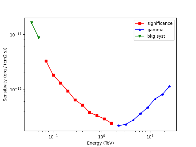
The results are given as an Astropy table. A column criterion allows to distinguish bins where the significance is limited by the signal statistical significance from bins where the sensitivity is limited by the number of signal counts. This is visible in the plot below.
# Show the results table
display(sensitivity_table)

# Save it to file (could use e.g. format of CSV or ECSV or FITS)
# sensitivity_table.write('sensitivity.ecsv', format='ascii.ecsv')

# Plot the sensitivity curve
t = sensitivity_table

is_s = t["criterion"] == "significance"

fig, ax = plt.subplots()
ax.plot(
    t["energy"][is_s],
    t["e2dnde"][is_s],
    "s-",
    color="red",
    label="significance",
)

is_g = t["criterion"] == "gamma"
ax.plot(t["energy"][is_g], t["e2dnde"][is_g], "*-", color="blue", label="gamma")
is_bkg_syst = t["criterion"] == "bkg"
ax.plot(
    t["energy"][is_bkg_syst],
    t["e2dnde"][is_bkg_syst],
    "v-",
    color="green",
    label="bkg syst",
)

ax.loglog()
ax.set_xlabel(f"Energy ({t['energy'].unit})")
ax.set_ylabel(f"Sensitivity ({t['e2dnde'].unit})")
ax.legend()
  energy      e2dnde     excess background  criterion
   TeV    erg / (cm2 s)
--------- ------------- ------- ---------- ------------
0.0356551   1.61512e-11 328.477    3284.77          bkg
0.0503641   8.66737e-12  165.06     1650.6          bkg
0.0711412   3.27253e-12 92.4984    756.756 significance
  0.10049   1.79729e-12 65.8637    376.563 significance
 0.141945   1.30282e-12 46.0027    178.563 significance
 0.200503   9.29846e-13 30.9746    77.2881 significance
 0.283218   6.38702e-13 21.3831    34.5112 significance
 0.400056   5.16894e-13 14.9743    15.4188 significance
 0.565095    3.7804e-13 11.0135    7.41691 significance
 0.798218    3.3034e-13 8.17611     3.4654 significance
  1.12751   2.89668e-13 6.53986    1.86033 significance
  1.59265   2.40531e-13 5.65742    1.19845 significance
  2.24968   2.16291e-13       5   0.743113        gamma
  3.17776   2.29643e-13       5   0.466104        gamma
  4.48871   2.73642e-13       5     0.3196        gamma
  6.34047   3.57511e-13       5    0.18669        gamma
  8.95615   4.65419e-13       5  0.0845693        gamma
  12.6509   6.65067e-13       5  0.0447552        gamma
  17.8699   7.96271e-13       5  0.0266192        gamma
  25.2419   1.12581e-12       5  0.0126585        gamma

<matplotlib.legend.Legend object at 0x7f8331bbb520>
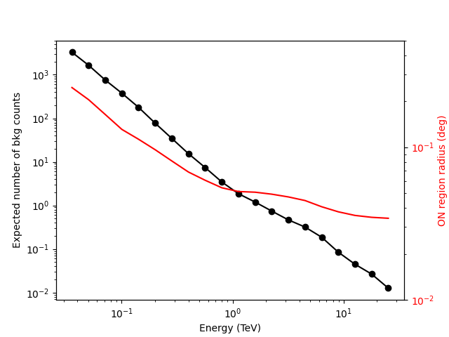
We add some control plots showing the expected number of background counts per bin and the ON region size cut (here the 68% containment radius of the PSF).
# Plot expected number of counts for signal and background
fig, ax1 = plt.subplots()
# ax1.plot( t["energy"], t["excess"],"o-", color="red", label="signal")
ax1.plot(t["energy"], t["background"], "o-", color="black", label="blackground")

ax1.loglog()
ax1.set_xlabel(f"Energy ({t['energy'].unit})")
ax1.set_ylabel("Expected number of bkg counts")

ax2 = ax1.twinx()
ax2.set_ylabel(f"ON region radius ({on_radii.unit})", color="red")
ax2.semilogy(t["energy"], on_radii, color="red", label="PSF68")
ax2.tick_params(axis="y", labelcolor="red")
ax2.set_ylim(0.01, 0.5)
plt.show()
Exercises#
Also compute the sensitivity for a 20 hour observation
Compare how the sensitivity differs between 5 and 20 hours by plotting the ratio as a function of energy.