VERITAS with Gammapy

Explore VERITAS point-like DL3 files, including event lists and IRFs and calculate Li & Ma significance, spectra, and fluxes.

Introduction

VERITAS (Very Energetic Radiation Imaging Telescope Array System) is a ground-based gamma-ray instrument operating at the Fred Lawrence Whipple Observatory (FLWO) in southern Arizona, USA. It is an array of four 12m optical reflectors for gamma-ray astronomy in the ~ 100 GeV to > 30 TeV energy range.

VERITAS data are private and lower level analysis is done using either the Eventdisplay or VEGAS (internal access only) analysis packages to produce DL3 files (using V2DL3), which can be used in Gammapy to produce high-level analysis products. A small sub-set of archival Crab nebula data has been publicly released to accompany this tutorial, which provides an introduction to VERITAS data analysis using gammapy for VERITAS members and external users alike.

This notebook is only intended for use with these publicly released Crab nebula files and the use of other sources or datasets may require modifications to this notebook.

import numpy as np
from matplotlib import pyplot as plt

import astropy.units as u

from gammapy.maps import MapAxis, WcsGeom, RegionGeom

from regions import CircleSkyRegion, PointSkyRegion
from gammapy.data import DataStore
from gammapy.modeling.models import SkyModel, LogParabolaSpectralModel
from gammapy.modeling import Fit
from gammapy.datasets import Datasets, SpectrumDataset
from gammapy.estimators import FluxPointsEstimator, LightCurveEstimator
from gammapy.makers import (
    ReflectedRegionsBackgroundMaker,
    SafeMaskMaker,
    SpectrumDatasetMaker,
    WobbleRegionsFinder,
)
from astropy.coordinates import SkyCoord
from gammapy.visualization import plot_spectrum_datasets_off_regions
from gammapy.utils.regions import extract_bright_star_regions

Data exploration

Load in files

First, we select and load VERITAS observations of the Crab Nebula. These files are processed with EventDisplay, but VEGAS analysis should be identical apart from the integration region size, which is handled by RAD_MAX.

data_store = DataStore.from_dir("$GAMMAPY_DATA/veritas/crab-point-like-ED")
data_store.info()

Data store:
HDU index table:
BASE_DIR: /home/runner/work/gammapy-docs/gammapy-docs/gammapy-datasets/2.0/veritas/crab-point-like-ED
Rows: 16
OBS_ID: 64080 -- 64083
HDU_TYPE: [np.str_('aeff'), np.str_('edisp'), np.str_('events'), np.str_('gti')]
HDU_CLASS: [np.str_('aeff_2d'), np.str_('edisp_2d'), np.str_('events'), np.str_('gti')]


Observation table:
Observatory name: 'N/A'
Number of observations: 4

We filter our data by only taking observations within \(5^\circ\) of the Crab Nebula. Further details on how to filter observations can be found in Data access and selection (DL3).

target_position = SkyCoord(83.6333, 22.0145, unit="deg")

selected_obs_table = data_store.obs_table.select_sky_circle(target_position, 5 * u.deg)
obs_ids = selected_obs_table["OBS_ID"]

observations = data_store.get_observations(obs_id=obs_ids, required_irf="point-like")

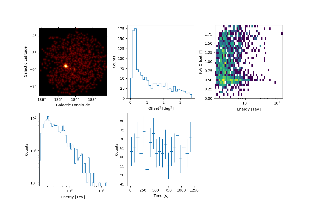
Peek the first run in the data release

Peek the events and their time/energy/spatial distributions.

observations[0].events.peek()
plt.show()

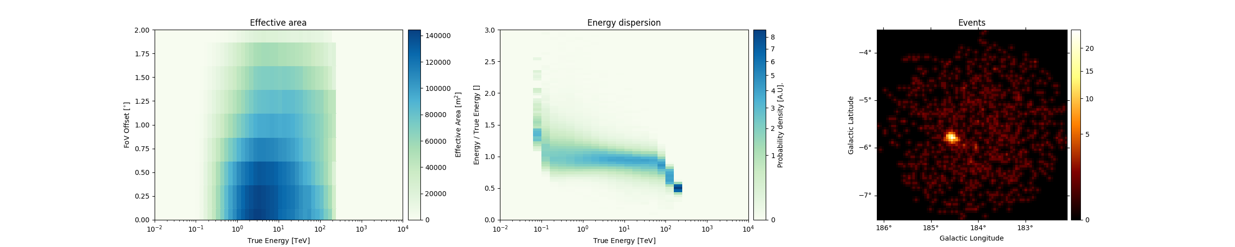
Peek at the IRFs included. You should verify that the IRFs are filled correctly and that there are no values set to zero within your analysis range. We can also peek at the effective area (aeff) or energy migration matrices (edisp) with the peek() method.

observations[0].peek(figsize=(25, 5))
plt.show()

Estimate counts and significance

Set the energy binning

The energy axis will determine the bins in which energy is calculated, while the true energy axis defines the binning of the energy dispersion matrix and the effective area. Generally, the true energy axis should be more finely binned than the energy axis and span a larger range of energies, and the energy axis should be binned to match the needs of spectral reconstruction.

Note that if the SafeMaskMaker (which we will define later) is set to exclude events below a given percentage of the effective area, it will remove the entire bin containing the energy that corresponds to that percentage. Additionally, spectral bins are determined based on the energy axis and cannot be finer or offset from the energy axis bin edges. See Safe Data Range for more information on how the safe mask maker works.

energy_axis = MapAxis.from_energy_bounds("0.05 TeV", "100 TeV", nbin=50)
energy_axis_true = MapAxis.from_energy_bounds(
    "0.01 TeV", "110 TeV", nbin=200, name="energy_true"
)

Create an exclusion mask

Here, we create a spatial mask and append exclusion regions for the source region and stars (< 6th magnitude) contained within the exclusion_geom. We define a star exclusion region of 0.3 deg, which should contain bright stars within the VERITAS optical PSF.

exclusion_geom = WcsGeom.create(
    skydir=(target_position.ra.value, target_position.dec.value),
    binsz=0.01,
    width=(4, 4),
    frame="icrs",
    proj="CAR",
)

source_exclusion_region = CircleSkyRegion(center=target_position, radius=0.35 * u.deg)
exclusion_regions = extract_bright_star_regions(exclusion_geom)
exclusion_regions.append(source_exclusion_region)

exclusion_mask = ~exclusion_geom.region_mask(exclusion_regions)

Define the integration region

Point-like DL3 files can only be analyzed using the reflected regions background method and for a pre-determined integration region (which is the \(\sqrt{\theta^2}\) used in IRF simulations).

The default values for moderate/medium cuts are determined by the DL3 file’s RAD_MAX keyword. For VERITAS data (ED and VEGAS), RAD_MAX is not energy dependent.

Note that full-enclosure files are required to use any non-point-like integration region.

on_region = PointSkyRegion(target_position)
geom = RegionGeom.create(region=on_region, axes=[energy_axis])

Define the SafeMaskMaker

The SafeMaskMaker sets the boundaries of our analysis based on the uncertainties contained in the instrument response functions (IRFs).

For VERITAS point-like analysis (both ED and VEGAS), the following methods are strongly recommended:

• offset-max: Sets the maximum radial offset from the camera center within which we accept events. This is set to the edge of the VERITAS FoV.

• edisp-bias: Removes events which are reconstructed with energies that have \(>5\%\) energy bias.

• aeff-max: Removes events which are reconstructed to \(<10\%\) of the maximum value of the effective area. These are important to remove for spectral analysis, since they have large uncertainties on their reconstructed energies.

safe_mask_maker = SafeMaskMaker(
    methods=["offset-max", "aeff-max", "edisp-bias"],
    aeff_percent=10,
    bias_percent=5,
    offset_max=1.75 * u.deg,
)

Data reduction

We will now run the data reduction chain to calculate our ON and OFF counts. To get a significance for the whole energy range (to match VERITAS packages), remove the SafeMaskMaker from being applied to dataset_on_off.

The parameters of the reflected background regions can be changed using the WobbleRegionsFinder, which is passed as an argument to the ReflectedRegionsBackgroundMaker.

dataset_maker = SpectrumDatasetMaker(selection=["counts", "exposure", "edisp"])
dataset_empty = SpectrumDataset.create(geom=geom, energy_axis_true=energy_axis_true)

region_finder = WobbleRegionsFinder(n_off_regions=16)
bkg_maker = ReflectedRegionsBackgroundMaker(
    exclusion_mask=exclusion_mask, region_finder=region_finder
)

datasets = Datasets()

for obs_id, observation in zip(obs_ids, observations):
    dataset = dataset_maker.run(dataset_empty.copy(name=str(obs_id)), observation)
    dataset = safe_mask_maker.run(dataset, observation)
    dataset_on_off = bkg_maker.run(dataset, observation)
    datasets.append(dataset_on_off)

The plot below will show your exclusion regions in black and the center of your background regions with coloured stars. You should check to make sure these regions are sensible and that none of your background regions overlap with your exclusion regions.

plt.figure()
ax = exclusion_mask.plot()
plot_spectrum_datasets_off_regions(ax=ax, datasets=datasets)
plt.show()

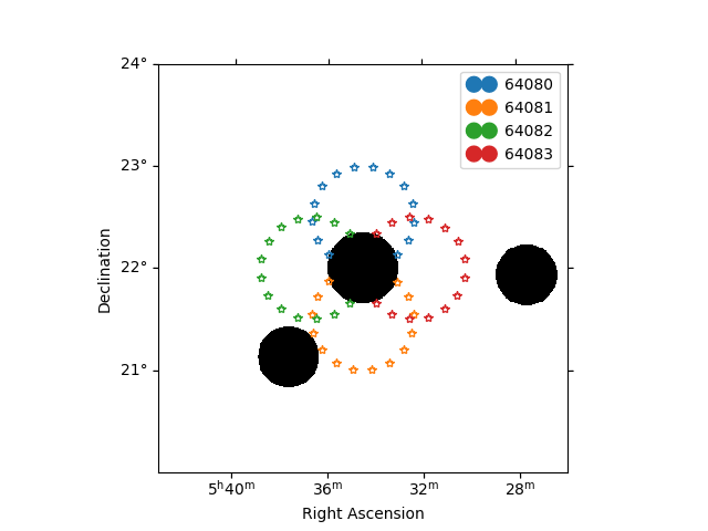
/home/runner/work/gammapy-docs/gammapy-docs/gammapy/.tox/build_docs/lib/python3.11/site-packages/gammapy/visualization/datasets.py:84: UserWarning: Setting the 'color' property will override the edgecolor or facecolor properties.
  handle = Patch(**plot_kwargs)

Significance analysis results

Here, we display the results of the significance analysis. info_table can be modified with cumulative = False to display a table with rows that correspond to the values for each run separately.

However, cumulative = True is needed to produce the combined values in the next cell.

info_table = datasets.info_table(cumulative=True)
print(info_table)

print(f"ON: {info_table['counts'][-1]}")
print(f"OFF: {info_table['counts_off'][-1]}")
print(f"Significance: {info_table['sqrt_ts'][-1]:.2f} sigma")
print(f"Alpha: {info_table['alpha'][-1]:.2f}")

  name  counts       excess       ...   acceptance_off         alpha
                                  ...
------- ------ ------------------ ... ------------------ ------------------
stacked    106 102.85713958740234 ...              560.0 0.0714285746216774
stacked    255 249.85714721679688 ...             1120.0 0.0714285746216774
stacked    383 375.78570556640625 ... 1679.9998779296875 0.0714285746216774
stacked    517 507.78570556640625 ...  2239.999755859375  0.071428582072258
ON: 517
OFF: 129
Significance: 46.60 sigma
Alpha: 0.07

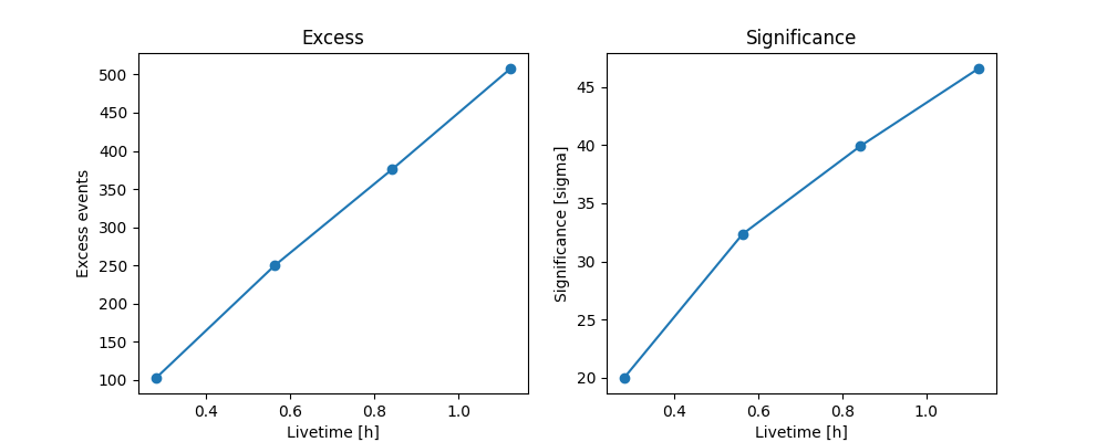
We can also plot the cumulative excess counts and significance over time. For a steady source, we generally expect excess to increase linearly with time and for significance to increase as \(\sqrt{\textrm{time}}\).

fig, (ax_excess, ax_sqrt_ts) = plt.subplots(figsize=(10, 4), ncols=2, nrows=1)
ax_excess.plot(
    info_table["livetime"].to("h"),
    info_table["excess"],
    marker="o",
)

ax_excess.set_title("Excess")
ax_excess.set_xlabel("Livetime [h]")
ax_excess.set_ylabel("Excess events")

ax_sqrt_ts.plot(
    info_table["livetime"].to("h"),
    info_table["sqrt_ts"],
    marker="o",
)

ax_sqrt_ts.set_title("Significance")
ax_sqrt_ts.set_xlabel("Livetime [h]")
ax_sqrt_ts.set_ylabel("Significance [sigma]")
plt.show()

Make a spectrum

Now, we’ll calculate the source spectrum. This uses a forward-folding approach that will assume a given spectrum and fit the counts calculated above to that spectrum in each energy bin specified by the energy_axis.

For this reason, it’s important that spectral model be set as closely as possible to the expected spectrum - for the Crab nebula, this is a LogParabolaSpectralModel.

spectral_model = LogParabolaSpectralModel(
    amplitude=3.75e-11 * u.Unit("cm-2 s-1 TeV-1"),
    alpha=2.45,
    beta=0.15,
    reference=1 * u.TeV,
)

model = SkyModel(spectral_model=spectral_model, name="crab")

datasets.models = [model]

fit_joint = Fit()
result_joint = fit_joint.run(datasets=datasets)

The best-fit spectral parameters are shown in this table.

print(datasets.models.to_parameters_table())

model type    name     value         unit      ... min max frozen link prior
----- ---- --------- ---------- -------------- ... --- --- ------ ---- -----
 crab      amplitude 4.0105e-11 TeV-1 s-1 cm-2 ... nan nan  False
 crab      reference 1.0000e+00            TeV ... nan nan   True
 crab          alpha 2.5289e+00                ... nan nan  False
 crab           beta 2.6446e-01                ... nan nan  False

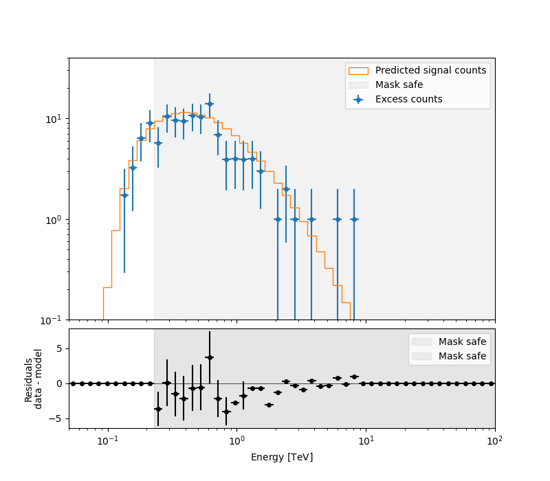
We can inspect how well our data fit the model’s predicted counts in each energy bin.

ax_spectrum, ax_residuals = datasets[0].plot_fit()
ax_spectrum.set_ylim(0.1, 40)
plt.show()

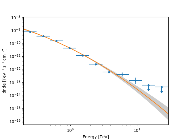
We can now calculate flux points to get a spectrum by fitting the result_joint model’s amplitude in selected energy bands (defined by energy_edges). We set selection_optional = "all" in FluxPointsEstimator, which will include a calculation for the upper limits in bins with a significance \(< 2\sigma\).

In the case of a non-detection or to obtain better upper limits, consider expanding the scan range for the norm parameter in FluxPointsEstimator. See Estimators for more details on how to do this.

fpe = FluxPointsEstimator(
    energy_edges=np.logspace(-0.7, 1.5, 12) * u.TeV,
    source="crab",
    selection_optional="all",
)
flux_points = fpe.run(datasets=datasets)

Now, we can plot our flux points along with the best-fit spectral model.

ax = flux_points.plot()
spectral_model.plot(ax=ax, energy_bounds=(0.1, 30) * u.TeV)
spectral_model.plot_error(ax=ax, energy_bounds=(0.1, 30) * u.TeV)

plt.show()

Make a lightcurve and calculate integral flux

Integral flux can be calculated by integrating the spectral model we fit earlier. This will be a model-dependent flux estimate, so the choice of spectral model should match the data as closely as possible.

e_min and e_max should be adjusted depending on the analysis requirements. Note that the actual energy threshold will use the closest bin defined by the energy_axis binning.

e_min = 0.25 * u.TeV
e_max = 30 * u.TeV

flux, flux_errp, flux_errn = result_joint.models["crab"].spectral_model.integral_error(
    e_min, e_max
)
print(
    f"Integral flux > {e_min}: {flux.value:.2} + {flux_errp.value:.2} {flux.unit} - {flux_errn.value:.2} {flux.unit}"
)

Integral flux > 0.25 TeV: 1.7e-10 + 8e-12 1 / (s cm2) - 8.3e-12 1 / (s cm2)

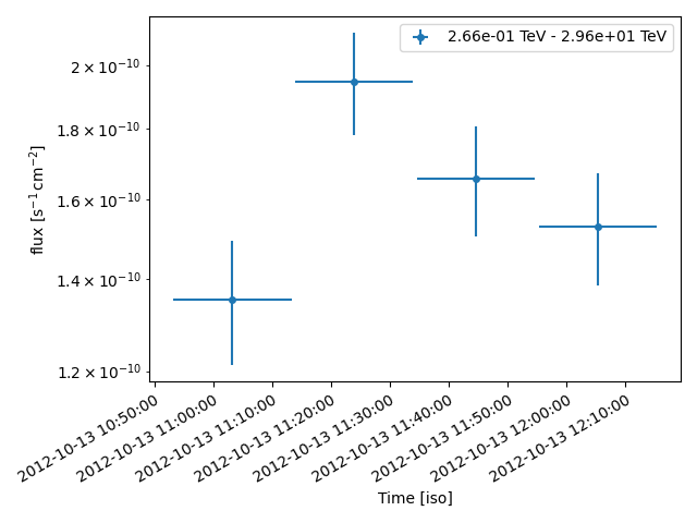
Finally, we’ll create a run-wise binned light curve. See the Light curves for flares tutorial for instructions on how to set up sub-run binning. Here, we set our energy edges so that the light curve has an energy threshold of 0.25 TeV and will plot upper limits for time bins with significance \(<2 \sigma\).

lc_maker = LightCurveEstimator(
    energy_edges=[0.25, 30] * u.TeV, source="crab", reoptimize=False
)
lc_maker.n_sigma_ul = 2
lc_maker.selection_optional = ["ul"]
lc = lc_maker.run(datasets)

We can look at our results by printing the light curve as a table (with each line corresponding to a light curve bin) and plotting the light curve.

fig, ax = plt.subplots()
lc.sqrt_ts_threshold_ul = 2
lc.plot(ax=ax, axis_name="time", sed_type="flux")
plt.tight_layout()

table = lc.to_table(format="lightcurve", sed_type="flux")
print(table["time_min", "time_max", "flux", "flux_err"])

     time_min           time_max      ...        flux_err
                                      ...      1 / (s cm2)
------------------ ------------------ ... ----------------------
 56213.45364922353 56213.467561260564 ... 1.3949943612472306e-11
 56213.46796520147 56213.481877238504 ...  1.652355175420978e-11
 56213.48233844736  56213.49625048439 ... 1.5247402003173758e-11
56213.496739178285  56213.51065121532 ...  1.432606578265409e-11