Spectrum simulation with Gammapy¶

Introduction¶

This notebook explains how to use the functions and classes in gammapy.spectrum in order to simulate and fit spectra.

First, we will simulate and fit a pure power law without any background. Than we will add a power law shaped background component. Finally, we will see how to simulate and fit a user defined model. For all scenarios a toy detector will be simulated. For an example using real CTA IRFs, checkout this notebook.

The following clases will be used:

Setup¶

Same procedure as in every script …

[1]:

%matplotlib inline
import matplotlib.pyplot as plt

[2]:

import numpy as np
import astropy.units as u
from gammapy.irf import EnergyDispersion, EffectiveAreaTable
from gammapy.spectrum import SpectrumSimulation, SpectrumFit
from gammapy.spectrum.models import PowerLaw

Create detector¶

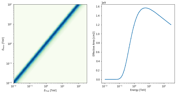
For the sake of self consistency of this tutorial, we will simulate a simple detector. For a real application you would want to replace this part of the code with loading the IRFs or your detector.

[3]:

e_true = np.logspace(-2, 2.5, 109) * u.TeV
e_reco = np.logspace(-2, 2, 79) * u.TeV

edisp = EnergyDispersion.from_gauss(
    e_true=e_true, e_reco=e_reco, sigma=0.2, bias=0
)
aeff = EffectiveAreaTable.from_parametrization(energy=e_true)

fig, axes = plt.subplots(1, 2, figsize=(12, 6))
edisp.plot_matrix(ax=axes[0])
aeff.plot(ax=axes[1]);

../_images/notebooks_spectrum_simulation_7_0.png

Power law¶

In this section we will simulate one observation using a power law model.

[4]:

pwl = PowerLaw(
    index=2.3, amplitude=1e-11 * u.Unit("cm-2 s-1 TeV-1"), reference=1 * u.TeV
)
print(pwl)

PowerLaw

Parameters:

           name     value   error      unit      min max frozen
        --------- --------- ----- -------------- --- --- ------
            index 2.300e+00   nan                nan nan  False
        amplitude 1.000e-11   nan cm-2 s-1 TeV-1 nan nan  False
        reference 1.000e+00   nan            TeV nan nan   True

[5]:

livetime = 2 * u.h
sim = SpectrumSimulation(
    aeff=aeff, edisp=edisp, source_model=pwl, livetime=livetime
)
sim.simulate_obs(seed=2309, obs_id=1)
print(sim.obs)

*** Observation summary report ***
Observation Id: 1
Livetime: 2.000 h
On events: 339
Off events: 0
Alpha: 1.000
Bkg events in On region: 0.00
Excess: 339.00
Gamma rate: 2.83 1 / min
Bkg rate: 0.00 1 / min
Sigma: nan
energy range: 0.01 TeV - 100.00 TeV

[6]:

fit = SpectrumFit(obs_list=sim.obs, model=pwl.copy(), stat="cash")
fit.fit_range = [1, 10] * u.TeV
fit.run()
print(fit.result[0])


Fit result info
---------------
Model: PowerLaw

Parameters:

           name     value     error        unit      min max frozen
        --------- --------- --------- -------------- --- --- ------
            index 2.259e+00 2.191e-01                nan nan  False
        amplitude 9.255e-12 1.754e-12 cm-2 s-1 TeV-1 nan nan  False
        reference 1.000e+00 0.000e+00            TeV nan nan   True

Covariance:

           name     index   amplitude reference
        --------- --------- --------- ---------
            index 4.802e-02 2.984e-13 0.000e+00
        amplitude 2.984e-13 3.077e-24 0.000e+00
        reference 0.000e+00 0.000e+00 0.000e+00

Statistic: -74.059 (cash)
Fit Range: [1.         9.42668455] TeV

Include background¶

In this section we will include a background component. Furthermore, we will also simulate more than one observation and fit each one individuallt in order to get average fit results.

[7]:

bkg_model = PowerLaw(
    index=2.5, amplitude=1e-11 * u.Unit("cm-2 s-1 TeV-1"), reference=1 * u.TeV
)

[8]:

%%time
n_obs = 30
seeds = np.arange(n_obs)

sim = SpectrumSimulation(
    aeff=aeff,
    edisp=edisp,
    source_model=pwl,
    livetime=livetime,
    background_model=bkg_model,
    alpha=0.2,
)

sim.run(seeds)
print(sim.result)
print(sim.result[0])

SpectrumObservationList
Number of observations: 30
*** Observation summary report ***
Observation Id: 0
Livetime: 2.000 h
On events: 733
Off events: 1915
Alpha: 0.200
Bkg events in On region: 383.00
Excess: 350.00
Excess / Background: 0.91
Gamma rate: 2.92 1 / min
Bkg rate: 0.04 1 / min
Sigma: 14.17
energy range: 0.01 TeV - 100.00 TeV
CPU times: user 298 ms, sys: 4.3 ms, total: 302 ms
Wall time: 151 ms

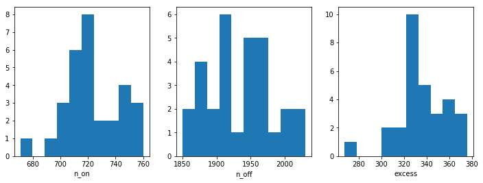
Before moving on to the fit let’s have a look at the simulated observations

[9]:

n_on = [obs.total_stats.n_on for obs in sim.result]
n_off = [obs.total_stats.n_off for obs in sim.result]
excess = [obs.total_stats.excess for obs in sim.result]

fix, axes = plt.subplots(1, 3, figsize=(12, 4))
axes[0].hist(n_on)
axes[0].set_xlabel("n_on")
axes[1].hist(n_off)
axes[1].set_xlabel("n_off")
axes[2].hist(excess)
axes[2].set_xlabel("excess");

../_images/notebooks_spectrum_simulation_16_0.png

[10]:

%%time
results = []
for obs in sim.result:
    fit = SpectrumFit(obs, pwl.copy(), stat="wstat")
    fit.optimize()
    results.append(
        {
            "index": fit.result[0].model.parameters["index"].value,
            "amplitude": fit.result[0].model.parameters["amplitude"].value,
        }
    )

CPU times: user 2.67 s, sys: 9.33 ms, total: 2.68 s
Wall time: 1.34 s

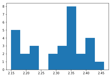
[11]:

index = np.array([_["index"] for _ in results])
plt.hist(index, bins=10)
print("spectral index: {:.2f} +/- {:.2f}".format(index.mean(), index.std()))

spectral index: 2.31 +/- 0.09

../_images/notebooks_spectrum_simulation_18_1.png

Exercises¶

Fit a pure power law and the user define model to the observation you just simulated. You can start with the user defined model described in the spectrum_models.ipynb notebook.
Vary the observation lifetime and see when you can distinguish the two models (Hint: You get the final likelihood of a fit from fit.result[0].statval).

What’s next¶

In this tutorial we learnd how to simulate and fit data using a toy detector. Go to gammapy.spectrum to see what else you can do with gammapy.