This is a fixed-text formatted version of a Jupyter notebook

Try online
You can contribute with your own notebooks in this GitHub repository.
Source files: analysis_3d.ipynb | analysis_3d.py

3D analysis¶

This tutorial does a 3D map based analsis on the galactic center, using simulated observations from the CTA-1DC. We will use the high level interface for the data reduction, and then do a detailed modelling. This will be done in two different ways:

stacking all the maps together and fitting the stacked maps
handling all the observations separately and doing a joint fitting on all the maps

[1]:

%matplotlib inline
import matplotlib.pyplot as plt
import astropy.units as u
from pathlib import Path
from regions import CircleSkyRegion
from gammapy.analysis import Analysis, AnalysisConfig
from gammapy.modeling.models import (
    SkyModel,
    ExpCutoffPowerLawSpectralModel,
    PointSpatialModel,
)
from gammapy.modeling import Fit
from gammapy.maps import Map

Analysis configuration¶

In this section we select observations and define the analysis geometries, irrespective of joint/stacked analysis. For configuration of the analysis, we will programatically build a config file from scratch.

[2]:

config = AnalysisConfig()
# The config file is now empty, with only a few defaults specified.
print(config)

AnalysisConfig

    general:
        log: {level: info, filename: null, filemode: null, format: null, datefmt: null}
        outdir: .
    observations:
        datastore: $GAMMAPY_DATA/hess-dl3-dr1
        obs_ids: []
        obs_file: null
        obs_cone: {frame: null, lon: null, lat: null, radius: null}
        obs_time: {start: null, stop: null}
    datasets:
        type: 1d
        stack: true
        geom:
            wcs:
                skydir: {frame: null, lon: null, lat: null}
                binsize: 0.02 deg
                fov: {width: 5.0 deg, height: 5.0 deg}
                binsize_irf: 0.2 deg
            selection: {offset_max: 2.5 deg}
            axes:
                energy: {min: 0.1 TeV, max: 10.0 TeV, nbins: 30}
                energy_true: {min: 0.1 TeV, max: 10.0 TeV, nbins: 30}
        map_selection: [counts, exposure, background, psf, edisp]
        background:
            method: null
            exclusion: null
            parameters: {}
        safe_mask:
            methods: [aeff-default]
            parameters: {}
        on_region: {frame: null, lon: null, lat: null, radius: null}
        containment_correction: true
    fit:
        fit_range: {min: 0.1 TeV, max: 10.0 TeV}
    flux_points:
        energy: {min: 0.1 TeV, max: 10.0 TeV, nbins: 30}
        source: source
        parameters: {}

[3]:

# Selecting the observations
config.observations.datastore = "$GAMMAPY_DATA/cta-1dc/index/gps/"
config.observations.obs_ids = [110380, 111140, 111159]

[4]:

# Defining a reference geometry for the reduced datasets

config.datasets.type = "3d"  # Analysis type is 3D

config.datasets.geom.wcs.skydir = {
    "lon": "0 deg",
    "lat": "0 deg",
    "frame": "galactic",
}  # The WCS geometry - centered on the galactic center
config.datasets.geom.wcs.fov = {"width": "10 deg", "height": "8 deg"}
config.datasets.geom.wcs.binsize = "0.02 deg"

# The FoV radius to use for cutouts
config.datasets.geom.selection.offset_max = 3.5 * u.deg
config.datasets.safe_mask.methods = ["aeff-default", "offset-max"]

# We now fix the energy axis for the counts map - (the reconstructed energy binning)
config.datasets.geom.axes.energy.min = "0.1 TeV"
config.datasets.geom.axes.energy.max = "10 TeV"
config.datasets.geom.axes.energy.nbins = 10

# We now fix the energy axis for the IRF maps (exposure, etc) - (the true enery binning)
config.datasets.geom.axes.energy_true.min = "0.08 TeV"
config.datasets.geom.axes.energy_true.max = "12 TeV"
config.datasets.geom.axes.energy_true.nbins = 14

[5]:

print(config)

AnalysisConfig

    general:
        log: {level: info, filename: null, filemode: null, format: null, datefmt: null}
        outdir: .
    observations:
        datastore: $GAMMAPY_DATA/cta-1dc/index/gps
        obs_ids: [110380, 111140, 111159]
        obs_file: null
        obs_cone: {frame: null, lon: null, lat: null, radius: null}
        obs_time: {start: null, stop: null}
    datasets:
        type: 3d
        stack: true
        geom:
            wcs:
                skydir: {frame: galactic, lon: 0.0 deg, lat: 0.0 deg}
                binsize: 0.02 deg
                fov: {width: 10.0 deg, height: 8.0 deg}
                binsize_irf: 0.2 deg
            selection: {offset_max: 3.5 deg}
            axes:
                energy: {min: 0.1 TeV, max: 10.0 TeV, nbins: 10}
                energy_true: {min: 0.08 TeV, max: 12.0 TeV, nbins: 14}
        map_selection: [counts, exposure, background, psf, edisp]
        background:
            method: null
            exclusion: null
            parameters: {}
        safe_mask:
            methods: [aeff-default, offset-max]
            parameters: {}
        on_region: {frame: null, lon: null, lat: null, radius: null}
        containment_correction: true
    fit:
        fit_range: {min: 0.1 TeV, max: 10.0 TeV}
    flux_points:
        energy: {min: 0.1 TeV, max: 10.0 TeV, nbins: 30}
        source: source
        parameters: {}

Configuration for stacked and joint analysis¶

This is done just by specfiying the flag on config.datasets.stack. Since the internal machinery will work differently for the two cases, we will write it as two config files and save it to disc in YAML format for future reference.

[6]:

config_stack = config.copy(deep=True)
config_stack.datasets.stack = True

config_joint = config.copy(deep=True)
config_joint.datasets.stack = False

[7]:

# To prevent unnecessary cluttering, we write it in a separate folder.
path = Path("analysis_3d")
path.mkdir(exist_ok=True)
config_joint.write(path=path / "config_joint.yaml", overwrite=True)
config_stack.write(path=path / "config_stack.yaml", overwrite=True)

Stacked analysis¶

Data reduction¶

We first show the steps for the stacked analysis and then repeat the same for the joint analysis later

[8]:

# Reading yaml file:
config_stacked = AnalysisConfig.read(path=path / "config_stack.yaml")

[9]:

analysis_stacked = Analysis(config_stacked)

Setting logging config: {'level': 'INFO', 'filename': None, 'filemode': None, 'format': None, 'datefmt': None}

[10]:

%%time
# select observations:
analysis_stacked.get_observations()

# run data reduction
analysis_stacked.get_datasets()

Fetching observations.
Number of selected observations: 3
Creating geometry.
Creating datasets.
No background maker set for 3d analysis. Check configuration.
Processing observation 110380
No thresholds defined for obs Observation

        obs id            : 110380
        tstart            : 59235.50
        tstop             : 59235.52
        duration          : 1800.00 s
        pointing (icrs)   : 267.7 deg, -29.6 deg

        deadtime fraction : 2.0%

Processing observation 111140
No thresholds defined for obs Observation

        obs id            : 111140
        tstart            : 59275.50
        tstop             : 59275.52
        duration          : 1800.00 s
        pointing (icrs)   : 264.2 deg, -29.5 deg

        deadtime fraction : 2.0%

Processing observation 111159
No thresholds defined for obs Observation

        obs id            : 111159
        tstart            : 59276.50
        tstop             : 59276.52
        duration          : 1800.00 s
        pointing (icrs)   : 266.0 deg, -27.0 deg

        deadtime fraction : 2.0%

CPU times: user 7.66 s, sys: 2.27 s, total: 9.93 s
Wall time: 10.3 s

We have one final dataset, which you can print and explore

[11]:

dataset_stacked = analysis_stacked.datasets["stacked"]
print(dataset_stacked)

MapDataset
----------

  Name                            : stacked

  Total counts                    : 121241
  Total predicted counts          : 108043.52
  Total background counts         : 108043.52

  Exposure min                    : 6.28e+07 m2 s
  Exposure max                    : 1.90e+10 m2 s

  Number of total bins            : 2000000
  Number of fit bins              : 1411180

  Fit statistic type              : cash
  Fit statistic value (-2 log(L)) : 625436.39

  Number of models                : 1
  Number of parameters            : 3
  Number of free parameters       : 1

  Component 0: BackgroundModel

    Name                      : stacked-bkg
    Datasets names            : ['stacked']
    Parameters:
      norm                    :   1.000
      tilt         (frozen)   :   0.000
      reference    (frozen)   :   1.000  TeV

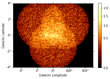
[12]:

# To plot a smooth counts map
dataset_stacked.counts.smooth(0.02 * u.deg).plot_interactive(add_cbar=True)

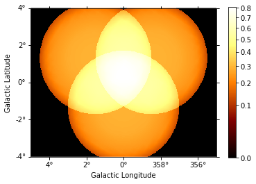
../_images/notebooks_analysis_3d_18_0.png

[13]:

# And the background map
dataset_stacked.background_model.map.plot_interactive(add_cbar=True)

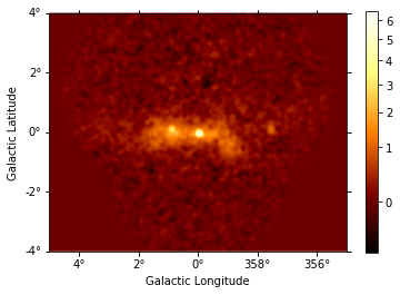
../_images/notebooks_analysis_3d_19_0.png

[14]:

# You can also get an excess image with a few lines of code:
counts = dataset_stacked.counts.sum_over_axes()
background = dataset_stacked.background_model.map.sum_over_axes()
excess = counts - background
excess.smooth("0.06 deg").plot(stretch="sqrt", add_cbar=True);

../_images/notebooks_analysis_3d_20_0.png

Modeling and fitting¶

Now comes the interesting part of the analysis - choosing appropriate models for our source and fitting them.

We choose a point source model with an exponential cutoff power-law spectrum.

To select a certain energy range for the fit we can create a fit mask:

[15]:

coords = dataset_stacked.counts.geom.get_coord()
mask_energy = coords["energy"] > 0.3 * u.TeV
dataset_stacked.mask_fit = Map.from_geom(
    geom=dataset_stacked.counts.geom, data=mask_energy
)

[16]:

spatial_model = PointSpatialModel(
    lon_0="-0.05 deg", lat_0="-0.05 deg", frame="galactic"
)
spectral_model = ExpCutoffPowerLawSpectralModel(
    index=2.3,
    amplitude=2.8e-12 * u.Unit("cm-2 s-1 TeV-1"),
    reference=1.0 * u.TeV,
    lambda_=0.02 / u.TeV,
)

model = SkyModel(
    spatial_model=spatial_model,
    spectral_model=spectral_model,
    name="gc-source",
)

dataset_stacked.models.append(model)
dataset_stacked.background_model.norm.value = 1.3

[17]:

%%time
fit = Fit([dataset_stacked])
result = fit.run(optimize_opts={"print_level": 1})

------------------------------------------------------------------
| FCN = 2.802E+05               |     Ncalls=177 (177 total)     |
| EDM = 9.39E-05 (Goal: 1E-05)  |            up = 1.0            |
------------------------------------------------------------------
|  Valid Min.   | Valid Param.  | Above EDM | Reached call limit |
------------------------------------------------------------------
|     True      |     True      |   False   |       False        |
------------------------------------------------------------------
| Hesse failed  |   Has cov.    | Accurate  | Pos. def. | Forced |
------------------------------------------------------------------
|     False     |     True      |   True    |   True    | False  |
------------------------------------------------------------------
CPU times: user 9.19 s, sys: 2.41 s, total: 11.6 s
Wall time: 11.7 s

[18]:

result.parameters.to_table()

[18]:

Table length=10

name	value	unit	min	max	frozen	error
str9	float64	str14	float64	float64	bool	float64
norm	1.248e+00		0.000e+00	nan	False	6.448e-03
tilt	0.000e+00		nan	nan	True	0.000e+00
reference	1.000e+00	TeV	nan	nan	True	0.000e+00
index	2.240e+00		nan	nan	False	1.146e-01
amplitude	2.909e-12	cm-2 s-1 TeV-1	nan	nan	False	3.341e-13
reference	1.000e+00	TeV	nan	nan	True	0.000e+00
lambda_	5.311e-02	TeV-1	nan	nan	False	6.112e-02
alpha	1.000e+00		nan	nan	True	0.000e+00
lon_0	-5.166e-02	deg	nan	nan	False	2.338e-03
lat_0	-5.244e-02	deg	-9.000e+01	9.000e+01	False	2.244e-03

Check model fit¶

We check the model fit by computing and plotting a residual image:

[19]:

dataset_stacked.plot_residuals(method="diff/sqrt(model)", vmin=-1, vmax=1)

[19]:

(<matplotlib.axes._subplots.WCSAxesSubplot at 0x116012c18>, None)

../_images/notebooks_analysis_3d_27_1.png

We can also plot the best fit spectrum. For that need to extract the covariance of the spectral parameters.

Joint analysis¶

In this section, we perform a joint analysis of the same data. Of course, joint fitting is considerably heavier than stacked one, and should always be handled with care. For brevity, we only show the analysis for a point source fitting without re-adding a diffuse component again.

Data reduction¶

[20]:

%%time

# Read the yaml file from disk
config_joint = AnalysisConfig.read(path=path / "config_joint.yaml")
analysis_joint = Analysis(config_joint)

# select observations:
analysis_joint.get_observations()

# run data reduction
analysis_joint.get_datasets()

Setting logging config: {'level': 'INFO', 'filename': None, 'filemode': None, 'format': None, 'datefmt': None}
Fetching observations.
Number of selected observations: 3
Creating geometry.
Creating datasets.
No background maker set for 3d analysis. Check configuration.
Processing observation 110380
No thresholds defined for obs Observation

        obs id            : 110380
        tstart            : 59235.50
        tstop             : 59235.52
        duration          : 1800.00 s
        pointing (icrs)   : 267.7 deg, -29.6 deg

        deadtime fraction : 2.0%

Processing observation 111140
No thresholds defined for obs Observation

        obs id            : 111140
        tstart            : 59275.50
        tstop             : 59275.52
        duration          : 1800.00 s
        pointing (icrs)   : 264.2 deg, -29.5 deg

        deadtime fraction : 2.0%

Processing observation 111159
No thresholds defined for obs Observation

        obs id            : 111159
        tstart            : 59276.50
        tstop             : 59276.52
        duration          : 1800.00 s
        pointing (icrs)   : 266.0 deg, -27.0 deg

        deadtime fraction : 2.0%

CPU times: user 6.94 s, sys: 1.97 s, total: 8.91 s
Wall time: 9.01 s

[21]:

# You can see there are 3 datasets now
print(analysis_joint.datasets)

Datasets
--------
idx=0, id='0x1180b8c18', name='-fbzIRNK'
idx=1, id='0x115ccf550', name='tk5xvVAM'
idx=2, id='0x115fc0080', name='1cpoqF7u'

[22]:

# You can access each one by name or by index, eg:
print(analysis_joint.datasets[0])

MapDataset
----------

  Name                            : -fbzIRNK

  Total counts                    : 47736
  Total predicted counts          : 42655.01
  Total background counts         : 42655.01

  Exposure min                    : 6.28e+07 m2 s
  Exposure max                    : 6.68e+09 m2 s

  Number of total bins            : 1085000
  Number of fit bins              : 693940

  Fit statistic type              : cash
  Fit statistic value (-2 log(L)) : 250423.04

  Number of models                : 1
  Number of parameters            : 3
  Number of free parameters       : 1

  Component 0: BackgroundModel

    Name                      : -fbzIRNK-bkg
    Datasets names            : ['-fbzIRNK']
    Parameters:
      norm                    :   1.000
      tilt         (frozen)   :   0.000
      reference    (frozen)   :   1.000  TeV

[23]:

# Add the model on each of the datasets
model_joint = model.copy(name="source-joint")
for dataset in analysis_joint.datasets:
    dataset.models.append(model_joint)
    dataset.background_model.norm.value = 1.1

[24]:

%%time
fit_joint = Fit(analysis_joint.datasets)
result_joint = fit_joint.run()

CPU times: user 27 s, sys: 5.37 s, total: 32.4 s
Wall time: 32.7 s

[25]:

print(result)

OptimizeResult

        backend    : minuit
        method     : minuit
        success    : True
        message    : Optimization terminated successfully.
        nfev       : 177
        total stat : 280219.84

[26]:

fit_joint.datasets.parameters.to_table()

[26]:

Table length=16

name	value	unit	min	max	frozen	error
str9	float64	str14	float64	float64	bool	float64
norm	1.117e+00		0.000e+00	nan	False	5.577e-03
tilt	0.000e+00		nan	nan	True	0.000e+00
reference	1.000e+00	TeV	nan	nan	True	0.000e+00
index	2.290e+00		nan	nan	False	7.647e-02
amplitude	2.885e-12	cm-2 s-1 TeV-1	nan	nan	False	3.116e-13
reference	1.000e+00	TeV	nan	nan	True	0.000e+00
lambda_	3.500e-02	TeV-1	nan	nan	False	5.131e-02
alpha	1.000e+00		nan	nan	True	0.000e+00
lon_0	-5.244e-02	deg	nan	nan	False	2.225e-03
lat_0	-5.247e-02	deg	-9.000e+01	9.000e+01	False	2.144e-03
norm	1.119e+00		0.000e+00	nan	False	5.580e-03
tilt	0.000e+00		nan	nan	True	0.000e+00
reference	1.000e+00	TeV	nan	nan	True	0.000e+00
norm	1.111e+00		0.000e+00	nan	False	5.561e-03
tilt	0.000e+00		nan	nan	True	0.000e+00
reference	1.000e+00	TeV	nan	nan	True	0.000e+00

The information which parameter belongs to which dataset is not listed explicitly in the table (yet), but the order of parameters is conserved. You can always access the underlying object tree as well to get specific parameter values:

[27]:

for dataset in analysis_joint.datasets:
    print(dataset.background_model.norm.value)

1.1172921144380115
1.1185249877971581
1.1111161210830067

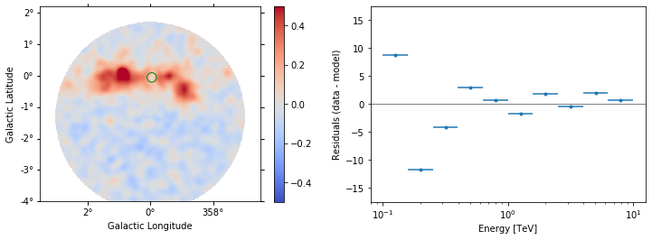
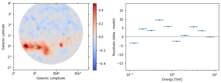
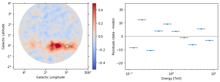
Residuals¶

Since we have multiple datasets, we can either look at a stacked residual map, or the residuals for each dataset. Each gammapy.cube.MapDataset object is equipped with a method called gammapy.cube.MapDataset.plot_residuals(), which displays the spatial and spectral residuals (computed as counts-model) for the dataset. Optionally, these can be normalized as (counts-model)/model or (counts-model)/sqrt(model), by passing the parameter norm='model or norm=sqrt_model.

[28]:

# To see the spectral residuals, we have to define a region for the spectral extraction
region = CircleSkyRegion(spatial_model.position, radius=0.15 * u.deg)

[29]:

for dataset in analysis_joint.datasets:
    ax_image, ax_spec = dataset.plot_residuals(
        region=region, vmin=-0.5, vmax=0.5, method="diff"
    )

../_images/notebooks_analysis_3d_41_0.png

../_images/notebooks_analysis_3d_41_1.png

../_images/notebooks_analysis_3d_41_2.png

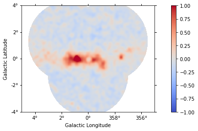
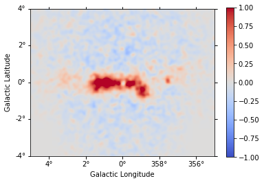
[30]:

# We need to stack on the full geometry, so we use to geom from the stacked counts map.
residuals_stacked = Map.from_geom(analysis_stacked.datasets[0].counts.geom)

for dataset in analysis_joint.datasets:
    residuals = dataset.residuals()
    residuals_stacked.stack(residuals)

residuals_stacked.sum_over_axes().smooth("0.08 deg").plot(
    vmin=-1, vmax=1, cmap="coolwarm", add_cbar=True, stretch="linear"
);

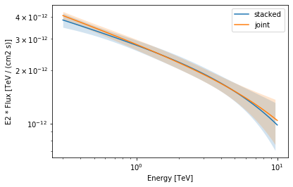
../_images/notebooks_analysis_3d_42_0.png

Finally let us compare the spectral results from the stacked and joint fit:

[31]:

def plot_spectrum(model, result, label, color):
    spec = model.spectral_model
    energy_range = [0.3, 10] * u.TeV
    spec.plot(
        energy_range=energy_range, energy_power=2, label=label, color=color
    )
    spec.plot_error(energy_range=energy_range, energy_power=2, color=color)

[32]:

plot_spectrum(model, result, label="stacked", color="tab:blue")
plot_spectrum(model_joint, result_joint, label="joint", color="tab:orange")
plt.legend()

[32]:

<matplotlib.legend.Legend at 0x115c96278>

../_images/notebooks_analysis_3d_45_1.png

Summary¶

Note that this notebook aims to show you the procedure of a 3D analysis using just a few observations. Results get much better for a more complete analysis considering the GPS dataset from the CTA First Data Challenge (DC-1) and also the CTA model for the Galactic diffuse emission, as shown in the next image:

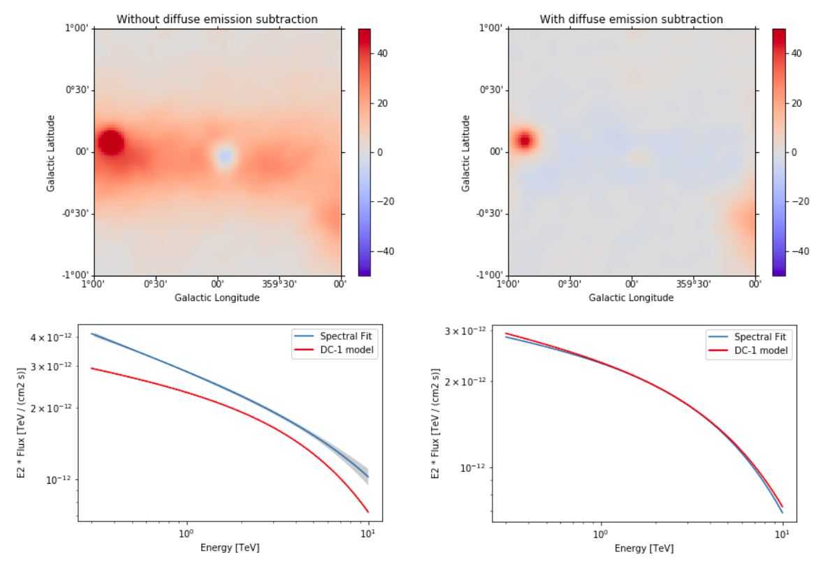
The complete tutorial notebook of this analysis is available to be downloaded in GAMMAPY-EXTRA repository at https://github.com/gammapy/gammapy-extra/blob/master/analyses/cta_1dc_gc_3d.ipynb).

Exercises¶

Analyse the second source in the field of view: G0.9+0.1 and add it to the combined model.
Perform modeling in more details - Add diffuse component, get flux points.