This is a fixed-text formatted version of a Jupyter notebook
Try online

You can contribute with your own notebooks in this GitHub repository.
Source files: analysis_mwl.ipynb | analysis_mwl.py
Joint modeling, fitting, and serialization
Prerequisites
Handling of Fermi-LAT data with gammapy see the corresponding tutorial
Knowledge of spectral analysis to produce 1D On-Off datasets, see the following tutorial
Using flux points to directly fit a model (without forward-folding) see the SED fitting tutorial
Context
Some science studies require to combine heterogeneous data from various instruments to extract physical informations. In particular, it is often useful to add flux measurements of a source at different energies to an analysis to better constrain the wide-band spectral parameters. This can be done using a joint fit of heterogeneous datasets.
Objectives: Constrain the spectral parameters of the gamma-ray emission from the Crab nebula between 10 GeV and 100 TeV, using a 3D Fermi dataset, a H.E.S.S. reduced spectrum and HAWC flux points.
Proposed approach
This tutorial illustrates how to perfom a joint modeling and fitting of the Crab Nebula spectrum using different datasets. The spectral parameters are optimized by combining a 3D analysis of Fermi-LAT data, a ON/OFF spectral analysis of HESS data, and flux points from HAWC.
In this tutorial we are going to use pre-made datasets. We prepared maps of the Crab region as seen by Fermi-LAT using the same event selection than the 3FHL catalog (7 years of data with energy from 10 GeV to 2 TeV). For the HESS ON/OFF analysis we used two observations from the first public data release with a significant signal from energy of about 600 GeV to 10 TeV. These observations have an offset of 0.5° and a zenith angle of 45-48°. The HAWC flux points data are taken from a recent analysis based on 2.5 years of data with energy between 300 Gev and 300 TeV.
The setup
[1]:
from astropy import units as u
import matplotlib.pyplot as plt
from gammapy.modeling import Fit
from gammapy.datasets import Datasets, FluxPointsDataset, SpectrumDatasetOnOff
from gammapy.estimators import (
    FluxPoints,
    FluxPointsEstimator,
)
from gammapy.maps import MapAxis
from pathlib import Path
Data and models files
The datasets serialization produce YAML files listing the datasets and models. In the following cells we show an example containning only the Fermi-LAT dataset and the Crab model.
Fermi-LAT-3FHL_datasets.yaml:
datasets:
- name: Fermi-LAT
  type: MapDataset
  likelihood: cash
  models:
- Crab Nebula
  background: background
  filename: $GAMMAPY_DATA/fermi-3fhl-crab/Fermi-LAT-3FHL_data_Fermi-LAT.fits
We used as model a point source with a log-parabola spectrum. The initial parameters were taken from the latest Fermi-LAT catalog 4FGL, then we have re-optimized the spectral parameters for our dataset in the 10 GeV - 2 TeV energy range (fixing the source position).
Fermi-LAT-3FHL_models.yaml:
components:
- name: Crab Nebula
  type: SkyModel
  spatial:
    type: PointSpatialModel
    frame: icrs
    parameters:
    - name: lon_0
      value: 83.63310241699219
      unit: deg
      min: .nan
      max: .nan
      frozen: true
    - name: lat_0
      value: 22.019899368286133
      unit: deg
      min: -90.0
      max: 90.0
      frozen: true
  spectral:
    type: LogParabolaSpectralModel
    parameters:
    - name: amplitude
      value: 0.3415498620816483
      unit: cm-2 s-1 TeV-1
      min: .nan
      max: .nan
      frozen: false
    - name: reference
      value: 5.054833602905273e-05
      unit: TeV
      min: .nan
      max: .nan
      frozen: true
    - name: alpha
      value: 2.510798031388936
      unit: ''
      min: .nan
      max: .nan
      frozen: false
    - name: beta
      value: -0.022476498188855533
      unit: ''
      min: .nan
      max: .nan
      frozen: false
- name: background
  type: BackgroundModel
  parameters:
  - name: norm
    value: 0.9544383244743555
    unit: ''
    min: 0.0
    max: .nan
    frozen: false
  - name: tilt
    value: 0.0
    unit: ''
    min: .nan
    max: .nan
    frozen: true
  - name: reference
    value: 1.0
    unit: TeV
    min: .nan
    max: .nan
    frozen: true
Reading different datasets
Fermi-LAT 3FHL: map dataset for 3D analysis
For now we let’s use the datasets serialization only to read the 3D MapDataset associated to Fermi-LAT 3FHL data and models.
[2]:
path = "$GAMMAPY_DATA/fermi-3fhl-crab/Fermi-LAT-3FHL"
filedata = Path(path + "_datasets.yaml")
filemodel = Path(path + "_models.yaml")
datasets = Datasets.read(filedata=filedata, filemodel=filemodel)
dataset_fermi = datasets[0]
[3]:
print(datasets[0].models)
Models

Component 0: SkyModel

  Name                      : Crab Nebula
  Datasets names            : None
  Spectral model type       : LogParabolaSpectralModel
  Spatial  model type       : PointSpatialModel
  Temporal model type       : None
  Parameters:
    amplitude               :   3.42e-01  1 / (cm2 s TeV)
    reference    (frozen)   :   0.000  TeV
    alpha                   :   2.511
    beta                    :  -0.022
    lon_0        (frozen)   :  83.633  deg
    lat_0        (frozen)   :  22.020  deg

Component 1: BackgroundModel

  Name                      : background
  Datasets names            : ['Fermi-LAT']
  Parameters:
    norm                    :   0.954
    tilt         (frozen)   :   0.000
    reference    (frozen)   :   1.000  TeV
We get the Crab model in order to share it with the other datasets
[4]:
crab_model = dataset_fermi.models["Crab Nebula"]
crab_spec = crab_model.spectral_model
print(crab_spec)
LogParabolaSpectralModel

   name     value         unit      min max frozen   error
--------- ---------- -------------- --- --- ------ ---------
amplitude  3.415e-01 cm-2 s-1 TeV-1 nan nan  False 0.000e+00
reference  5.055e-05            TeV nan nan   True 0.000e+00
    alpha  2.511e+00                nan nan  False 0.000e+00
     beta -2.248e-02                nan nan  False 0.000e+00
HESS-DL3: 1D ON/OFF dataset for spectral fitting
The ON/OFF datasets can be read from PHA files following the OGIP standards. We read the PHA files from each observation, and compute a stacked dataset for simplicity. Then the Crab spectral model previously defined is added to the dataset.
[5]:
datasets = []

for obs_id in [23523, 23526]:
    dataset = SpectrumDatasetOnOff.from_ogip_files(
        f"$GAMMAPY_DATA/joint-crab/spectra/hess/pha_obs{obs_id}.fits"
    )
    datasets.append(dataset)

dataset_hess = Datasets(datasets).stack_reduce(name="HESS")
dataset_hess.models = crab_model
/Users/terrier/Code/gammapy-dev/gammapy-docs/build/v0.17/gammapy/gammapy/utils/interpolation.py:163: RuntimeWarning: overflow encountered in log
  return np.log(values)
HAWC: 1D dataset for flux point fitting
The HAWC flux point are taken from https://arxiv.org/pdf/1905.12518.pdf. Then these flux points are read from a pre-made FITS file and passed to a FluxPointsDataset together with the source spectral model.
[6]:
# read flux points from https://arxiv.org/pdf/1905.12518.pdf
filename = "$GAMMAPY_DATA/hawc_crab/HAWC19_flux_points.fits"
flux_points_hawc = FluxPoints.read(filename)
dataset_hawc = FluxPointsDataset(crab_model, flux_points_hawc, name="HAWC")
Datasets serialization
The datasets object contains each dataset previously defined. It can be saved on disk as datasets.yaml, models.yaml, and several data files specific to each dataset. Then the datasets can be rebuild later from these files.
[7]:
datasets = Datasets([dataset_fermi, dataset_hess, dataset_hawc])
path = Path("crab-3datasets")
path.mkdir(exist_ok=True)

datasets.write(path=path, prefix="crab_10GeV_100TeV", overwrite=True)
filedata = path / "crab_10GeV_100TeV_datasets.yaml"
filemodel = path / "crab_10GeV_100TeV_models.yaml"
datasets = Datasets.read(filedata=filedata, filemodel=filemodel)
[8]:
print(datasets["HESS"].models)
Models

Component 0: SkyModel

  Name                      : Crab Nebula
  Datasets names            : None
  Spectral model type       : LogParabolaSpectralModel
  Spatial  model type       : PointSpatialModel
  Temporal model type       : None
  Parameters:
    amplitude               :   3.42e-01  1 / (cm2 s TeV)
    reference    (frozen)   :   0.000  TeV
    alpha                   :   2.511
    beta                    :  -0.022
    lon_0        (frozen)   :  83.633  deg
    lat_0        (frozen)   :  22.020  deg

Component 1: BackgroundModel

  Name                      : background
  Datasets names            : ['Fermi-LAT']
  Parameters:
    norm                    :   0.954
    tilt         (frozen)   :   0.000
    reference    (frozen)   :   1.000  TeV
Joint analysis
We run the fit on the Datasets object that include a dataset for each instrument
[9]:
%%time
fit_joint = Fit(datasets)
results_joint = fit_joint.run()
print(results_joint)
print(results_joint.parameters.to_table())
OptimizeResult

        backend    : minuit
        method     : minuit
        success    : True
        message    : Optimization terminated successfully.
        nfev       : 829
        total stat : -14819.11

   name     value        unit         min        max    frozen   error
--------- --------- -------------- ---------- --------- ------ ---------
amplitude 4.015e-03 cm-2 s-1 TeV-1        nan       nan  False 1.072e-04
reference 5.055e-05            TeV        nan       nan   True 0.000e+00
    alpha 1.260e+00                       nan       nan  False 7.101e-04
     beta 6.185e-02                       nan       nan  False 1.962e-04
    lon_0 8.363e+01            deg        nan       nan   True 0.000e+00
    lat_0 2.202e+01            deg -9.000e+01 9.000e+01   True 0.000e+00
     norm 9.839e-01                 0.000e+00       nan  False 3.239e-01
     tilt 0.000e+00                       nan       nan   True 0.000e+00
reference 1.000e+00            TeV        nan       nan   True 0.000e+00
CPU times: user 12.6 s, sys: 105 ms, total: 12.7 s
Wall time: 12.7 s
Let’s display only the parameters of the Crab spectral model
[10]:
crab_spec = datasets[0].models["Crab Nebula"].spectral_model
print(crab_spec)
LogParabolaSpectralModel

   name     value        unit      min max frozen   error
--------- --------- -------------- --- --- ------ ---------
amplitude 4.015e-03 cm-2 s-1 TeV-1 nan nan  False 1.072e-04
reference 5.055e-05            TeV nan nan   True 0.000e+00
    alpha 1.260e+00                nan nan  False 7.101e-04
     beta 6.185e-02                nan nan  False 1.962e-04
We can compute flux points for Fermi-LAT and HESS datasets in order plot them together with the HAWC flux point.
[11]:
# compute Fermi-LAT and HESS flux points
e_edges = MapAxis.from_bounds(
    0.01, 2.0, nbin=6, interp="log", unit="TeV"
).edges

flux_points_fermi = FluxPointsEstimator(
    e_edges=e_edges, source="Crab Nebula"
).run([dataset_fermi])


e_edges = MapAxis.from_bounds(1, 15, nbin=6, interp="log", unit="TeV").edges
flux_points_hess = FluxPointsEstimator(
    e_edges=e_edges, source="Crab Nebula"
).run([dataset_hess])
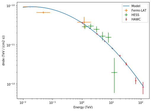
Now, Let’s plot the Crab spectrum fitted and the flux points of each instrument.
[12]:
# display spectrum and flux points
energy_range = [0.01, 120] * u.TeV
plt.figure(figsize=(8, 6))
ax = crab_spec.plot(energy_range=energy_range, energy_power=2, label="Model")
crab_spec.plot_error(ax=ax, energy_range=energy_range, energy_power=2)
flux_points_fermi.plot(ax=ax, energy_power=2, label="Fermi-LAT")
flux_points_hess.plot(ax=ax, energy_power=2, label="HESS")
flux_points_hawc.plot(ax=ax, energy_power=2, label="HAWC")
plt.legend();
[ ]: