Period detection and plotting
Introduction
time provides methods for period detection in time series, i.e. light
curves of \(\gamma\)-ray sources. The period detection is implemented in the
scope of the Lomb-Scargle periodogram, a method that detects periods in unevenly
sampled time series typical for \(\gamma\)-ray observations. We refer to the
astropy.timeseries.LombScargle-class and documentation within for an introduction
to the Lomb-Scargle algorithm, interpretation and usage 1.
With robust_periodogram, the analysis is extended to a more
general case where the unevenly sampled time series is contaminated by outliers,
i.e. due to the source’s high states. This robust periodogram includes the naive
Lomb-Scargle implementation as a special case.
robust_periodogram returns the periodogram of the input. This is
done by fitting a single sinusoidal model to the light curve and computing a
normalised \(\chi^2\)-statistic for each period of interest. The
Lomb-Scargle algorithm uses a naive least square regression and thus, is
sensitive to outliers in the light curve. Contrary,
robust_periodogram uses different loss functions that account
for outliers 2. The location of the highest periodogram peak is assumed to be
the period of an intrinsic periodic behaviour.
The result’s significance can be estimated in terms of a false alarm probability
(FAP) with the respective function of the astropy.timeseries.LombScargle-class. It
computes the probability of the highest periodogram peak being observed by
chance if the underlying light curve would consist of Gaussian white-noise only.
Both, periodogram and light curve can be plotted with
plot_periodogram.
See the Astropy docs for more details about the Lomb-Scargle periodogram and
its false alarm probability 1. The loss functions for the robust periodogram
are provided by scipy.optimize.least_squares 2.
Getting Started
Basic Usage
robust_periodogram takes a light curve with data format time
and flux as input. It returns the period grid, the periodogram peaks and the
location of the highest periodogram peak.
>>> import numpy as np
>>> from gammapy.time import robust_periodogram
>>> time = np.linspace(0.1, 10, 100)
>>> flux = np.sin(2 * np.pi * time)
>>> periodogram = robust_periodogram(time, flux)
>>> periodogram['best_period']
0.99
The returned period diverges from the true period of \(P = 1\), since this
period is not contained in the linear period grid automatically computed by
robust_periodogram.
Period Grid
The checked periods can be specified optionally by forwarding an array
periods.
>>> periods = np.linspace(0.1, 10, 100)
>>> periodogram = robust_periodogram(time, flux, periods=periods)
>>> periodogram['best_period']
1.0
If not given, a linear grid will be computed limited by the length of the light curve and the Nyquist frequency.
Measurement Uncertainties
robust_periodogram can also handle measurement uncertainties.
They can be forwarded as an array flux_err.
>>> rand = np.random.RandomState(42)
>>> flux_err = 0.1 * rand.rand(100)
>>> periodogram = robust_periodogram(time, flux, flux_err=flux_err, periods=periods)
>>> periodogram['best_period']
1.0
Loss Function and Loss Scale
To obtain a robust periodogram, loss function loss and loss scale parameter
scale need to be given.
>>> periodogram = robust_periodogram(time, flux, loss='huber', scale=1)
For available parameters, see 2. The choice of loss and scale depends
on the data set and needs to be optimised by the user.
If the loss function linear is used, robust_periodogram is
performed with an ordinary linear least square regression. It is then identical
to astropy.timeseries.LombScargle and scale can be set arbitrarily. This is the
default setting.
>>> from astropy.timeseries import LombScargle
>>> periods = np.linspace(1.1, 10, 90)
>>> periodogram = robust_periodogram(time, flux, periods=periods)
>>> LSP = LombScargle(time, flux).power(1. / periods)
>>> np.isclose(periodogram['power'], LSP).all() == True
True
Also, if scale is set to infinity, this results in the Lomb-Scargle
periodogram for any loss. Default settings are recommended if no outliers
are expected in the light curve.
False Alarm Probabilities
For the determination of peak significance in terms of a false alarm
probability, see 1 and 7. Methods for the false alarm probability can be
chosen from methods 3. The respective modul can be called, for example
with the Baluev-method:
>>> from astropy.timeseries.lombscargle import _statistics
>>> periods = np.linspace(0.1, 10, 100)
>>> periodogram = robust_periodogram(time, flux, periods=periods)
>>> fap = _statistics.false_alarm_probability(
...     periodogram['power'].max(), 1. / periodogram['periods'].min(),
...     time, flux, flux_err, 'standard', 'baluev'
... )
>>> fap
0.0
If other loss functions than linear are used, using the Bootstrap-method
is not recommended, because it internally calls astropy.timeseries.LombScargle
(linear least square regression) which is not identical to non-linear robust
periodogram.
Plotting
For plotting, plot_periodogram can be used. It takes the output
of robust_periodogram as input.
>>> import matplotlib.pyplot as plt
>>> from gammapy.time import plot_periodogram
>>> fig = plot_periodogram(
...     time, flux, periodogram['periods'], periodogram['power'],
...     flux_err, periodogram['best_period'], fap
... )
>>> fig.show()
Example
An example of detecting a period with robust_periodogram is
shown in the figure below. The code can be found under 4. The light curve of
the X-ray binary LS 5039 is used, observed in 2005 with H.E.S.S. at energies
above \(0.1 \mathrm{TeV}\) 4. The robust periodogram reveals the period
of \(P = (3.907 \pm 0.001) \mathrm{d}\) in agreement with 5 and 6.
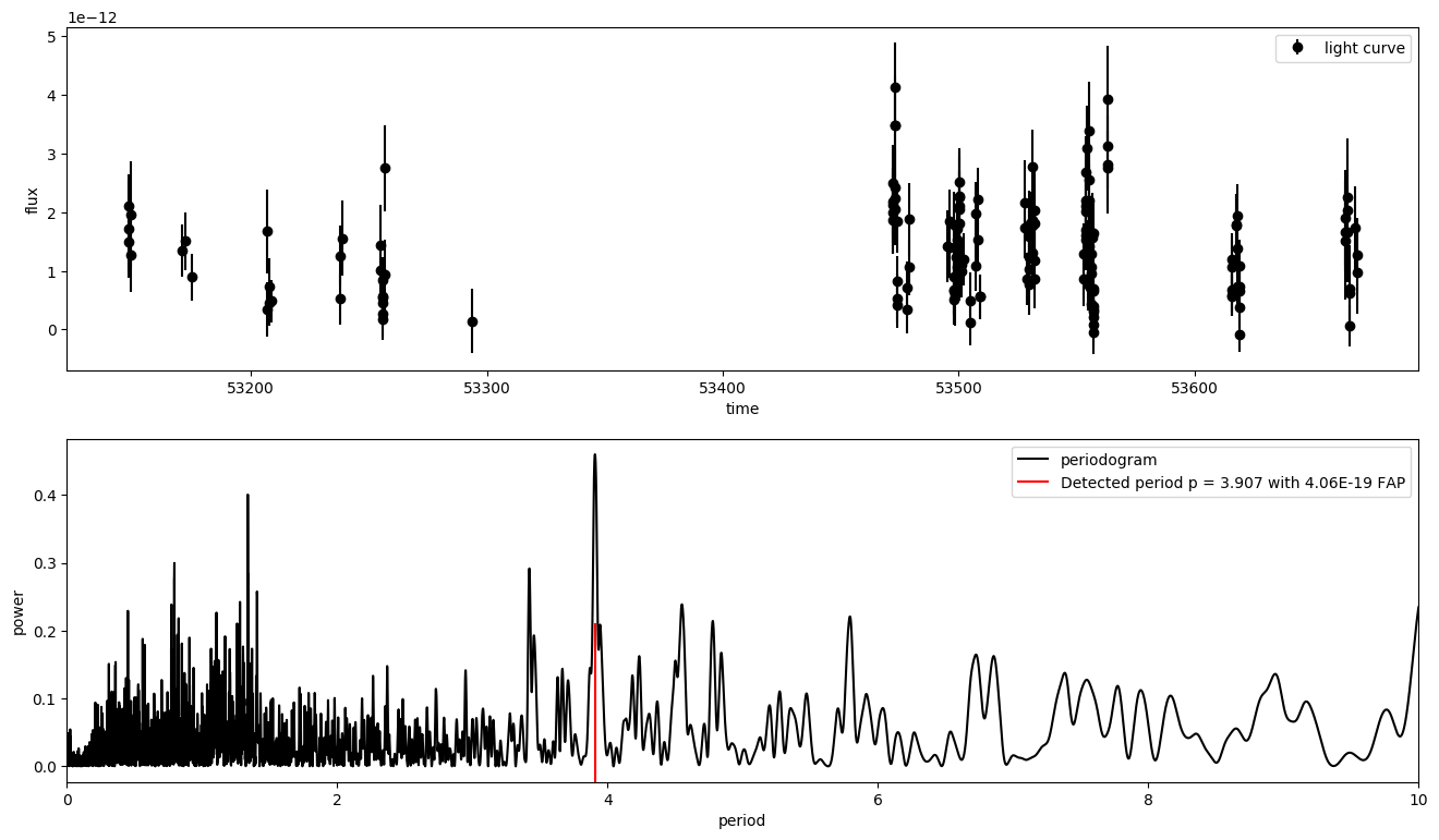
The maximum FAP of the highest periodogram peak is estimated to \(4.06e^{-19}\) with the \(\texttt{Baluev}\)-method. The other methods return following FAP:
method |
FAP |
|---|---|
‘single’ |
\(1.04e^{-21}\) |
‘naive’ |
\(5.40e^{-16}\) |
‘davies’ |
\(4.05e^{-15}\) |
‘baluev’ |
\(4.05e^{-15}\) |
‘bootstrap’ |
\(0.0\) |
The plot of the light curve shows no evidence for outliers. Thus,
\(\texttt{linear}\) is used as loss with an arbitrary scale of
\(1\). As periods, a linear grid is forwarded that is limited by \(10
\mathrm{d}\) to decrease computation time in favour for a higher resolution of
\(0.001 \mathrm{d}\).
The periodogram has many spurious peaks, which are due to several factors:
Errors in observations lead to leakage of power from the true peaks.
The signal is not a perfect sinusoid, so additional peaks can indicate higher-frequency components in the signal.
Sampling biases the periodogram and leads to failure modes. Its impact can be qualified by the spectral window function. This is the periodogram of the observation window and can be computed by setting
fluxandflux errto one and runningastropy.timeseries.LombScargle.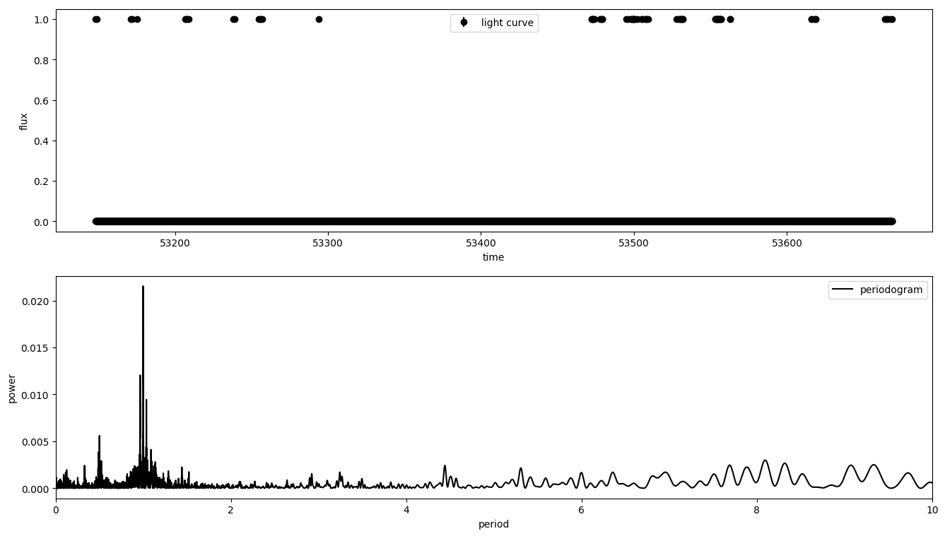
It shows a prominent peak around one day that arises from the nightly observation cycle. Aliases in the light curve’s periodogram, \(P_{{alias}}\), are expected to appear at \(f_{{true}} + n f_{{window}}\). In terms of periods
\[P_{{alias}} = (\frac{{1}}{{P_{true}}} + n f_{{window}})^{{-1}}\]for integer values of \(n\) 7. For the peak in the spectral window function at \(f_{{window}} = 0.997 d^{{-1}}\), this corresponds to the third highest peak in the periodogram at \(P_{{alias}} = 0.794\).
- 1(1,2,3)
Astropy docs, Lomb-Scargle Periodograms, Link
- 2(1,2,3)
Scipy docs, scipy.optimize.least_squares Link
- 3
Astropy docs, Utilities for computing periodogram statistics. Link
- 4(1,2)
Gammapy docs, period detection example, Link
- 5
F. Aharonian, 3.9 day orbital modulation in the TeV gamma-ray flux and spectrum from the X-ray binary LS 5039, Link
- 6
J. Casares, A possible black hole in the gamma-ray microquasar LS 5039, Link
- 7(1,2)
Jacob T. VanderPlas, Understanding the Lomb-Scargle Periodogram, Link