This is a fixed-text formatted version of a Jupyter notebook
Try online

You may download all the notebooks as a tar file.
Source files: modeling_2D.ipynb | modeling_2D.py
2D map fitting#
Prerequisites#
To understand how a generel modelling and fiiting works in gammapy, please refer to the analysis_3d tutorial
Context#
We often want the determine the position and morphology of an object. To do so, we don’t necessarily have to resort to a full 3D fitting but can perform a simple image fitting, in particular, in an energy range where the PSF does not vary strongly, or if we want to explore a possible energy dependence of the morphology.
Objective#
To localize a source and/or constrain its morphology.
Proposed approach#
The first step here, as in most analysis with DL3 data, is to create reduced datasets. For this, we will use the Analysis class to create a single set of stacked maps with a single bin in energy (thus, an image which behaves as a cube). This, we will then model with a spatial model of our choice, while keeping the spectral model fixed to an integrated power law.
Setup#
As usual, we’ll start with some general imports…
[1]:
%matplotlib inline
import astropy.units as u
from astropy.coordinates import SkyCoord
from astropy.time import Time

import logging

log = logging.getLogger(__name__)
Now let’s import gammapy specific classes and functions
[2]:
from gammapy.analysis import Analysis, AnalysisConfig
Creating the config file#
Now, we create a config file for out analysis. You may load this from disc if you have a pre-defined config file.
Here, we use 3 simulated CTA runs of the galactic center.
[3]:
config = AnalysisConfig()
# Selecting the observations
config.observations.datastore = "$GAMMAPY_DATA/cta-1dc/index/gps/"
config.observations.obs_ids = [110380, 111140, 111159]
Technically, gammapy implements 2D analysis as a special case of 3D analysis (one one bin in energy). So, we must specify the type of analysis as 3D, and define the geometry of the analysis.
[4]:
config.datasets.type = "3d"
config.datasets.geom.wcs.skydir = {
    "lon": "0 deg",
    "lat": "0 deg",
    "frame": "galactic",
}  # The WCS geometry - centered on the galactic center
config.datasets.geom.wcs.width = {"width": "8 deg", "height": "6 deg"}
config.datasets.geom.wcs.binsize = "0.02 deg"

# The FoV radius to use for cutouts
config.datasets.geom.selection.offset_max = 2.5 * u.deg
config.datasets.safe_mask.methods = ["offset-max"]
config.datasets.safe_mask.parameters = {"offset_max": 2.5 * u.deg}
config.datasets.background.method = "fov_background"
config.fit.fit_range = {"min": "0.1 TeV", "max": "30.0 TeV"}

# We now fix the energy axis for the counts map - (the reconstructed energy binning)
config.datasets.geom.axes.energy.min = "0.1 TeV"
config.datasets.geom.axes.energy.max = "10 TeV"
config.datasets.geom.axes.energy.nbins = 1

config.datasets.geom.wcs.binsize_irf = 0.2 * u.deg
[5]:
print(config)
AnalysisConfig

    general:
        log: {level: info, filename: null, filemode: null, format: null, datefmt: null}
        outdir: .
        n_jobs: 1
        datasets_file: null
        models_file: null
    observations:
        datastore: $GAMMAPY_DATA/cta-1dc/index/gps
        obs_ids: [110380, 111140, 111159]
        obs_file: null
        obs_cone: {frame: null, lon: null, lat: null, radius: null}
        obs_time: {start: null, stop: null}
        required_irf: [aeff, edisp, psf, bkg]
    datasets:
        type: 3d
        stack: true
        geom:
            wcs:
                skydir: {frame: galactic, lon: 0.0 deg, lat: 0.0 deg}
                binsize: 0.02 deg
                width: {width: 8.0 deg, height: 6.0 deg}
                binsize_irf: 0.2 deg
            selection: {offset_max: 2.5 deg}
            axes:
                energy: {min: 0.1 TeV, max: 10.0 TeV, nbins: 1}
                energy_true: {min: 0.5 TeV, max: 20.0 TeV, nbins: 16}
        map_selection: [counts, exposure, background, psf, edisp]
        background:
            method: fov_background
            exclusion: null
            parameters: {}
        safe_mask:
            methods: [offset-max]
            parameters: {offset_max: 2.5 deg}
        on_region: {frame: null, lon: null, lat: null, radius: null}
        containment_correction: true
    fit:
        fit_range: {min: 0.1 TeV, max: 30.0 TeV}
    flux_points:
        energy: {min: null, max: null, nbins: null}
        source: source
        parameters: {selection_optional: all}
    excess_map:
        correlation_radius: 0.1 deg
        parameters: {}
        energy_edges: {min: null, max: null, nbins: null}
    light_curve:
        time_intervals: {start: null, stop: null}
        energy_edges: {min: null, max: null, nbins: null}
        source: source
        parameters: {selection_optional: all}
Getting the reduced dataset#
We now use the config file and create a single MapDataset containing counts, background, exposure, psf and edisp maps.
[6]:
%%time
analysis = Analysis(config)
analysis.get_observations()
analysis.get_datasets()
Setting logging config: {'level': 'INFO', 'filename': None, 'filemode': None, 'format': None, 'datefmt': None}
Fetching observations.
Observations selected: 3 out of 3.
Number of selected observations: 3
Creating reference dataset and makers.
Creating the background Maker.
Start the data reduction loop.
Computing dataset for observation 110380
Running MapDatasetMaker
Invalid unit found in background table! Assuming (s-1 MeV-1 sr-1)
Running SafeMaskMaker
Running FoVBackgroundMaker
Computing dataset for observation 111140
Running MapDatasetMaker
Invalid unit found in background table! Assuming (s-1 MeV-1 sr-1)
Running SafeMaskMaker
Running FoVBackgroundMaker
Computing dataset for observation 111159
Running MapDatasetMaker
Invalid unit found in background table! Assuming (s-1 MeV-1 sr-1)
Running SafeMaskMaker
Running FoVBackgroundMaker
CPU times: user 5.35 s, sys: 1.04 s, total: 6.38 s
Wall time: 8.63 s
[7]:
print(analysis.datasets["stacked"])
MapDataset
----------

  Name                            : stacked

  Total counts                    : 85625
  Total background counts         : 85624.99
  Total excess counts             : 0.01

  Predicted counts                : 85625.00
  Predicted background counts     : 85624.99
  Predicted excess counts         : nan

  Exposure min                    : 8.46e+08 m2 s
  Exposure max                    : 2.14e+10 m2 s

  Number of total bins            : 120000
  Number of fit bins              : 96602

  Fit statistic type              : cash
  Fit statistic value (-2 log(L)) : nan

  Number of models                : 0
  Number of parameters            : 0
  Number of free parameters       : 0
The counts and background maps have only one bin in reconstructed energy. The exposure and IRF maps are in true energy, and hence, have a different binning based upon the binning of the IRFs. We need not bother about them presently.
[8]:
analysis.datasets["stacked"].counts
[8]:
WcsNDMap

        geom  : WcsGeom
        axes  : ['lon', 'lat', 'energy']
        shape : (400, 300, 1)
        ndim  : 3
        unit  :
        dtype : float32
[9]:
analysis.datasets["stacked"].background
[9]:
WcsNDMap

        geom  : WcsGeom
        axes  : ['lon', 'lat', 'energy']
        shape : (400, 300, 1)
        ndim  : 3
        unit  :
        dtype : float32
[10]:
analysis.datasets["stacked"].exposure
[10]:
WcsNDMap

        geom  : WcsGeom
        axes  : ['lon', 'lat', 'energy_true']
        shape : (400, 300, 16)
        ndim  : 3
        unit  : m2 s
        dtype : float32
We can have a quick look of these maps in the following way:
[11]:
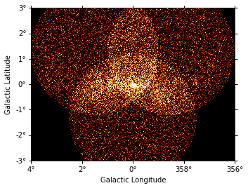
analysis.datasets["stacked"].counts.reduce_over_axes().plot(vmax=5)
[11]:
<WCSAxesSubplot:xlabel='Galactic Longitude', ylabel='Galactic Latitude'>
Modelling#
Now, we define a model to be fitted to the dataset. The important thing to note here is the dummy spectral model - an integrated powerlaw with only free normalisation. Here, we use its YAML definition to load it:
[12]:
model_config = """
components:
- name: GC-1
  type: SkyModel
  spatial:
    type: PointSpatialModel
    frame: galactic
    parameters:
    - name: lon_0
      value: 0.02
      unit: deg
    - name: lat_0
      value: 0.01
      unit: deg
  spectral:
    type: PowerLaw2SpectralModel
    parameters:
    - name: amplitude
      value: 1.0e-12
      unit: cm-2 s-1
    - name: index
      value: 2.0
      unit: ''
      frozen: true
    - name: emin
      value: 0.1
      unit: TeV
      frozen: true
    - name: emax
      value: 10.0
      unit: TeV
      frozen: true
"""
[13]:
analysis.set_models(model_config)
Reading model.
Models

Component 0: SkyModel

  Name                      : GC-1
  Datasets names            : None
  Spectral model type       : PowerLaw2SpectralModel
  Spatial  model type       : PointSpatialModel
  Temporal model type       :
  Parameters:
    amplitude                     :   1.00e-12   +/- 0.0e+00 1 / (cm2 s)
    index                 (frozen):      2.000
    emin                  (frozen):      0.100       TeV
    emax                  (frozen):     10.000       TeV
    lon_0                         :      0.020   +/-    0.00 deg
    lat_0                         :      0.010   +/-    0.00 deg

Component 1: FoVBackgroundModel

  Name                      : stacked-bkg
  Datasets names            : ['stacked']
  Spectral model type       : PowerLawNormSpectralModel
  Parameters:
    norm                          :      1.000   +/-    0.00
    tilt                  (frozen):      0.000
    reference             (frozen):      1.000       TeV
We will freeze the parameters of the background
[14]:
analysis.datasets["stacked"].background_model.parameters["tilt"].frozen = True
[15]:
# To run the fit
analysis.run_fit()
Fitting datasets.
OptimizeResult

        backend    : minuit
        method     : migrad
        success    : True
        message    : Optimization terminated successfully.
        nfev       : 184
        total stat : 170089.04

CovarianceResult

        backend    : minuit
        method     : hesse
        success    : True
        message    : Hesse terminated successfully.
[16]:
# To see the best fit values along with the errors
analysis.models.to_parameters_table()
[16]:
| model | type | name | value | unit | error | min | max | frozen | is_norm | link |
|---|---|---|---|---|---|---|---|---|---|---|
| str11 | str8 | str9 | float64 | str8 | float64 | float64 | float64 | bool | bool | str1 |
| GC-1 | spectral | amplitude | 4.1800e-11 | cm-2 s-1 | 2.231e-12 | nan | nan | False | True | |
| GC-1 | spectral | index | 2.0000e+00 | 0.000e+00 | nan | nan | True | False | ||
| GC-1 | spectral | emin | 1.0000e-01 | TeV | 0.000e+00 | nan | nan | True | False | |
| GC-1 | spectral | emax | 1.0000e+01 | TeV | 0.000e+00 | nan | nan | True | False | |
| GC-1 | spatial | lon_0 | -5.4767e-02 | deg | 1.993e-03 | nan | nan | False | False | |
| GC-1 | spatial | lat_0 | -5.3629e-02 | deg | 1.981e-03 | -9.000e+01 | 9.000e+01 | False | False | |
| stacked-bkg | spectral | norm | 9.9438e-01 | 3.411e-03 | nan | nan | False | True | ||
| stacked-bkg | spectral | tilt | 0.0000e+00 | 0.000e+00 | nan | nan | True | False | ||
| stacked-bkg | spectral | reference | 1.0000e+00 | TeV | 0.000e+00 | nan | nan | True | False |
[ ]: