This is a fixed-text formatted version of a Jupyter notebook
Try online

You may download all the notebooks as a tar file.
Source files: datasets.ipynb | datasets.py
Datasets - Reduced data, IRFs, models#
Introduction#
gammapy.datasets are a crucial part of the gammapy API. datasets constitute DL4 data - binned counts, IRFs, models and the associated likelihoods. Datasets from the end product of the makers stage, see makers notebook, and are passed on to the Fit or estimator classes for modelling and fitting purposes.
To find the different types of Dataset that are supported see Datasets home
Setup#
[1]:
import numpy as np
import astropy.units as u
from astropy.time import Time
from regions import CircleSkyRegion
from astropy.coordinates import SkyCoord
from gammapy.datasets import (
    MapDataset,
    SpectrumDataset,
    SpectrumDatasetOnOff,
    Datasets,
    FluxPointsDataset,
)
from gammapy.data import DataStore, GTI
from gammapy.maps import WcsGeom, RegionGeom, MapAxes, MapAxis, Map
from gammapy.modeling.models import (
    SkyModel,
    PowerLawSpectralModel,
    FoVBackgroundModel,
)
from gammapy.estimators import FluxPoints
from gammapy.utils.scripts import make_path
[2]:
%matplotlib inline
MapDataset#
The counts, exposure, background, masks, and IRF maps are bundled together in a data structure named MapDataset. While the counts, and background maps are binned in reconstructed energy and must have the same geometry, the IRF maps can have a different spatial (coarsely binned and larger) geometry and spectral range (binned in true energies). It is usually recommended that the true energy bin should be larger and more finely sampled and the reco energy bin.
Creating an empty dataset#
An empty MapDataset can be directly instantiated from any WcsGeom object:
[3]:
energy_axis = MapAxis.from_energy_bounds(
    1, 10, nbin=11, name="energy", unit="TeV"
)

geom = WcsGeom.create(
    skydir=(83.63, 22.01),
    axes=[energy_axis],
    width=5 * u.deg,
    binsz=0.05 * u.deg,
    frame="icrs",
)

dataset_empty = MapDataset.create(geom=geom, name="my-dataset")
It is good practice to define a name for the dataset, such that you can identify it later by name. However if you define a name it must be unique. Now we can already print the dataset:
[4]:
print(dataset_empty)
MapDataset
----------

  Name                            : my-dataset

  Total counts                    : 0
  Total background counts         : 0.00
  Total excess counts             : 0.00

  Predicted counts                : 0.00
  Predicted background counts     : 0.00
  Predicted excess counts         : nan

  Exposure min                    : 0.00e+00 m2 s
  Exposure max                    : 0.00e+00 m2 s

  Number of total bins            : 110000
  Number of fit bins              : 0

  Fit statistic type              : cash
  Fit statistic value (-2 log(L)) : nan

  Number of models                : 0
  Number of parameters            : 0
  Number of free parameters       : 0
The printout shows the key summary information of the dataset, such as total counts, fit statistics, model information etc.
MapDataset.from_geom has additional keywords, that can be used to define the binning of the IRF related maps:
[5]:
# choose a different true energy binning for the exposure, psf and edisp
energy_axis_true = MapAxis.from_energy_bounds(
    0.1, 100, nbin=11, name="energy_true", unit="TeV", per_decade=True
)

# choose a different rad axis binning for the psf
rad_axis = MapAxis.from_bounds(0, 5, nbin=50, unit="deg", name="rad")

gti = GTI.create(0 * u.s, 1000 * u.s)

dataset_empty = MapDataset.create(
    geom=geom,
    energy_axis_true=energy_axis_true,
    rad_axis=rad_axis,
    binsz_irf=0.1,
    gti=gti,
    name="dataset-empty",
)
To see the geometry of each map, we can use:
[6]:
dataset_empty.geoms
[6]:
{'geom': WcsGeom

        axes       : ['lon', 'lat', 'energy']
        shape      : (100, 100, 11)
        ndim       : 3
        frame      : icrs
        projection : CAR
        center     : 83.6 deg, 22.0 deg
        width      : 5.0 deg x 5.0 deg
        wcs ref    : 83.6 deg, 22.0 deg,
 'geom_exposure': WcsGeom

        axes       : ['lon', 'lat', 'energy_true']
        shape      : (100, 100, 33)
        ndim       : 3
        frame      : icrs
        projection : CAR
        center     : 83.6 deg, 22.0 deg
        width      : 5.0 deg x 5.0 deg
        wcs ref    : 83.6 deg, 22.0 deg,
 'geom_psf': WcsGeom

        axes       : ['lon', 'lat', 'rad', 'energy_true']
        shape      : (50, 50, 50, 33)
        ndim       : 4
        frame      : icrs
        projection : CAR
        center     : 83.6 deg, 22.0 deg
        width      : 5.0 deg x 5.0 deg
        wcs ref    : 83.6 deg, 22.0 deg,
 'geom_edisp': WcsGeom

        axes       : ['lon', 'lat', 'energy', 'energy_true']
        shape      : (50, 50, 11, 33)
        ndim       : 4
        frame      : icrs
        projection : CAR
        center     : 83.6 deg, 22.0 deg
        width      : 5.0 deg x 5.0 deg
        wcs ref    : 83.6 deg, 22.0 deg}
Another way to create a MapDataset is to just read an existing one from a FITS file:
[7]:
dataset_cta = MapDataset.read(
    "$GAMMAPY_DATA/cta-1dc-gc/cta-1dc-gc.fits.gz", name="dataset-cta"
)
[8]:
print(dataset_cta)
MapDataset
----------

  Name                            : dataset-cta

  Total counts                    : 104317
  Total background counts         : 91507.70
  Total excess counts             : 12809.30

  Predicted counts                : 91507.69
  Predicted background counts     : 91507.70
  Predicted excess counts         : nan

  Exposure min                    : 6.28e+07 m2 s
  Exposure max                    : 1.90e+10 m2 s

  Number of total bins            : 768000
  Number of fit bins              : 691680

  Fit statistic type              : cash
  Fit statistic value (-2 log(L)) : nan

  Number of models                : 0
  Number of parameters            : 0
  Number of free parameters       : 0
Accessing contents of a dataset#
To further explore the contents of a Dataset, you can use e.g. .info_dict()
[9]:
# For a quick info, use
dataset_cta.info_dict()
[9]:
{'name': 'dataset-cta',
 'counts': 104317,
 'excess': 12809.3046875,
 'sqrt_ts': 41.41009347393684,
 'background': 91507.6953125,
 'npred': 91507.68628538586,
 'npred_background': 91507.6953125,
 'npred_signal': nan,
 'exposure_min': <Quantity 62842028. m2 s>,
 'exposure_max': <Quantity 1.90242058e+10 m2 s>,
 'livetime': <Quantity 5292.00010298 s>,
 'ontime': <Quantity 5400. s>,
 'counts_rate': <Quantity 19.71220672 1 / s>,
 'background_rate': <Quantity 17.29170324 1 / s>,
 'excess_rate': <Quantity 2.42050348 1 / s>,
 'n_bins': 768000,
 'n_fit_bins': 691680,
 'stat_type': 'cash',
 'stat_sum': nan}
[10]:
# For a quick view, use
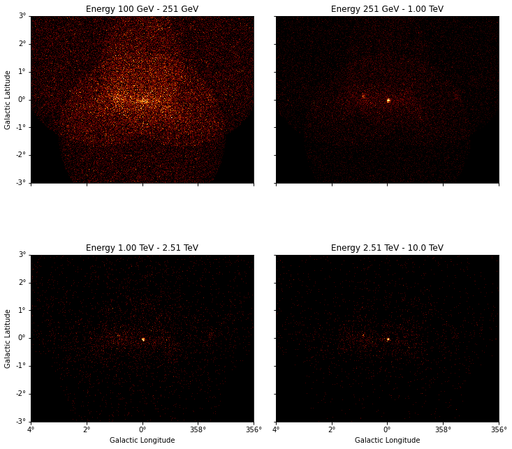
dataset_cta.peek()
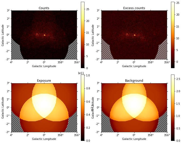
And access individual maps like:
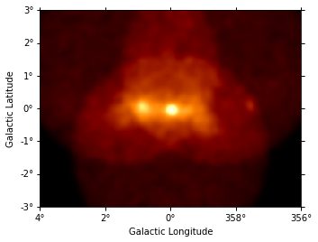
[11]:
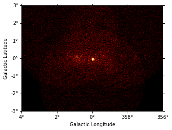
counts_image = dataset_cta.counts.sum_over_axes()
counts_image.smooth("0.1 deg").plot()
[11]:
<WCSAxesSubplot:xlabel='Galactic Longitude', ylabel='Galactic Latitude'>
Of course you can also access IRF related maps, e.g. the psf as PSFMap:
[12]:
dataset_cta.psf
[12]:
<gammapy.irf.psf.map.PSFMap at 0x168219d90>
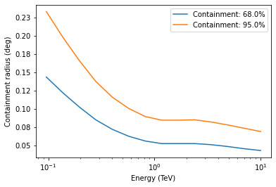
And use any method on the PSFMap object:
[13]:
dataset_cta.psf.plot_containment_radius_vs_energy()
[13]:
<AxesSubplot:xlabel='Energy (TeV)', ylabel='Containment radius (deg)'>
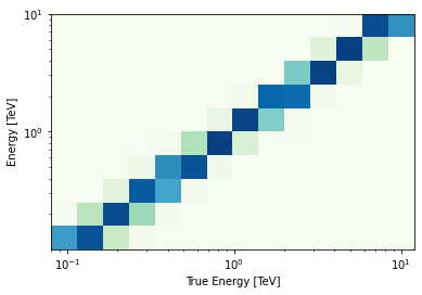
[14]:
edisp_kernel = dataset_cta.edisp.get_edisp_kernel()
edisp_kernel.plot_matrix()
[14]:
<AxesSubplot:xlabel='True Energy [TeV]', ylabel='Energy [TeV]'>
The MapDataset typically also contains the information on the residual hadronic background, stored in MapDataset.background as a map:
[15]:
dataset_cta.background
[15]:
WcsNDMap

        geom  : WcsGeom
        axes  : ['lon', 'lat', 'energy']
        shape : (320, 240, 10)
        ndim  : 3
        unit  :
        dtype : >f4
As a next step we define a minimal model on the dataset using the .models setter:
[16]:
model = SkyModel.create("pl", "point", name="gc")
model.spatial_model.position = SkyCoord("0d", "0d", frame="galactic")
model_bkg = FoVBackgroundModel(dataset_name="dataset-cta")

dataset_cta.models = [model, model_bkg]
Assigning models to datasets is covered in more detail in the Modeling notebook. Printing the dataset will now show the mode components:
[17]:
print(dataset_cta)
MapDataset
----------

  Name                            : dataset-cta

  Total counts                    : 104317
  Total background counts         : 91507.70
  Total excess counts             : 12809.30

  Predicted counts                : 91719.65
  Predicted background counts     : 91507.69
  Predicted excess counts         : 211.96

  Exposure min                    : 6.28e+07 m2 s
  Exposure max                    : 1.90e+10 m2 s

  Number of total bins            : 768000
  Number of fit bins              : 691680

  Fit statistic type              : cash
  Fit statistic value (-2 log(L)) : 424648.57

  Number of models                : 2
  Number of parameters            : 8
  Number of free parameters       : 5

  Component 0: SkyModel

    Name                      : gc
    Datasets names            : None
    Spectral model type       : PowerLawSpectralModel
    Spatial  model type       : PointSpatialModel
    Temporal model type       :
    Parameters:
      index                         :      2.000   +/-    0.00
      amplitude                     :   1.00e-12   +/- 0.0e+00 1 / (cm2 s TeV)
      reference             (frozen):      1.000       TeV
      lon_0                         :      4.650   +/-    0.00 rad
      lat_0                         :     -0.505   +/-    0.00 rad

  Component 1: FoVBackgroundModel

    Name                      : dataset-cta-bkg
    Datasets names            : ['dataset-cta']
    Spectral model type       : PowerLawNormSpectralModel
    Parameters:
      norm                          :      1.000   +/-    0.00
      tilt                  (frozen):      0.000
      reference             (frozen):      1.000       TeV
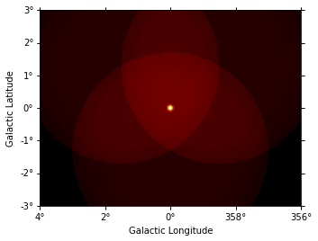
Now we can use .npred() to get a map of the total predicted counts of the model:
[18]:
npred = dataset_cta.npred()
npred.sum_over_axes().plot()
[18]:
<WCSAxesSubplot:xlabel='Galactic Longitude', ylabel='Galactic Latitude'>
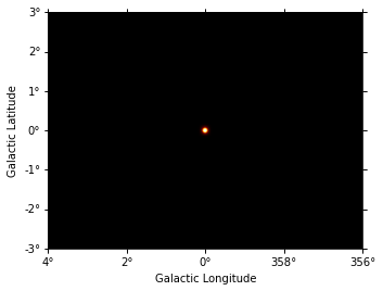
To get the predicted counts from an individual model component we can use:
[19]:
npred_source = dataset_cta.npred_signal(model_name="gc")
npred_source.sum_over_axes().plot()
[19]:
<WCSAxesSubplot:xlabel='Galactic Longitude', ylabel='Galactic Latitude'>
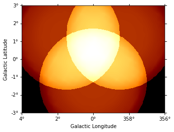
MapDataset.background contains the background map computed from the IRF. Internally it will be combined with a FoVBackgroundModel, to allow for adjusting the backgroun model during a fit. To get the model corrected background, one can use dataset.npred_background().
[20]:
npred_background = dataset_cta.npred_background()
npred_background.sum_over_axes().plot()
[20]:
<WCSAxesSubplot:xlabel='Galactic Longitude', ylabel='Galactic Latitude'>
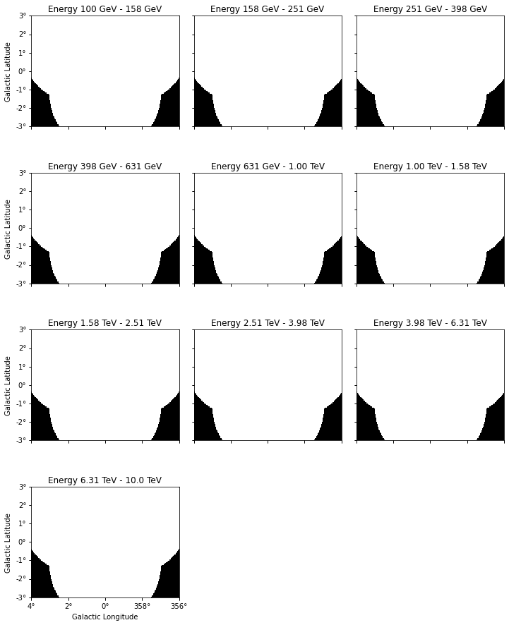
Using masks#
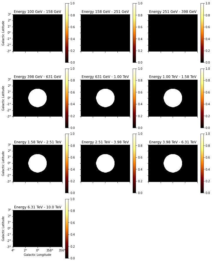
There are two masks that can be set on a Dataset, mask_safe and mask_fit.
The
mask_safeis computed during the data reduction process according to the specified selection cuts, and should not be changed by the user.During modelling and fitting, the user might want to additionally ignore some parts of a reduced dataset, e.g. to restrict the fit to a specific energy range or to ignore parts of the region of interest. This should be done by applying the
mask_fit. To see details of applying masks, please refer to Masks-for-fitting
Both the mask_fit and mask_safe must have the safe geom as the counts and background maps.
[21]:
# eg: to see the safe data range
dataset_cta.mask_safe.plot_grid();
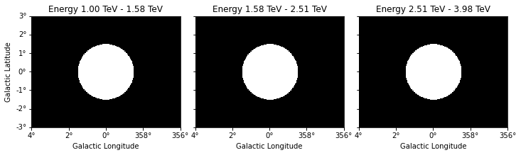
In addition it is possible to define a custom mask_fit:
[22]:
# To apply a mask fit - in enegy and space
region = CircleSkyRegion(SkyCoord("0d", "0d", frame="galactic"), 1.5 * u.deg)

geom = dataset_cta.counts.geom

mask_space = geom.region_mask([region])
mask_energy = geom.energy_mask(0.3 * u.TeV, 8 * u.TeV)
dataset_cta.mask_fit = mask_space & mask_energy
dataset_cta.mask_fit.plot_grid(vmin=0, vmax=1, add_cbar=True);
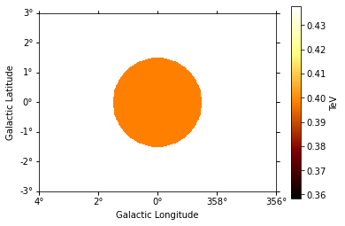
To access the energy range defined by the mask you can use: - dataset.energy_range_safe : energy range definedby the mask_safe - dataset.energy_range_fit : energy range defined by the mask_fit - dataset.energy_range : the final energy range used in likelihood computation
These methods return two maps, with the min and max energy values at each spatial pixel
[23]:
e_min, e_max = dataset_cta.energy_range
[24]:
# To see the lower energy threshold at each point
e_min.plot(add_cbar=True)
[24]:
<WCSAxesSubplot:xlabel='Galactic Longitude', ylabel='Galactic Latitude'>
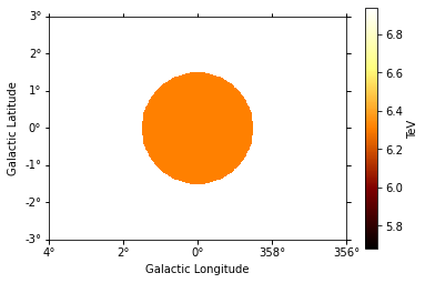
[25]:
# To see the lower energy threshold at each point
e_max.plot(add_cbar=True)
[25]:
<WCSAxesSubplot:xlabel='Galactic Longitude', ylabel='Galactic Latitude'>
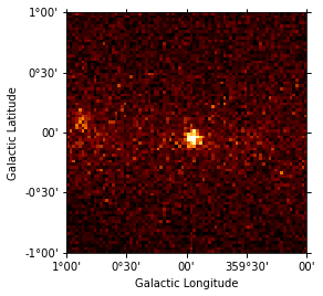
Just as for Map objects it is possible to cutout a whole MapDataset, which will perform the cutout for all maps in parallel.Optionally one can provide a new name to the resulting dataset:
[26]:
cutout = dataset_cta.cutout(
    position=SkyCoord("0d", "0d", frame="galactic"),
    width=2 * u.deg,
    name="cta-cutout",
)
[27]:
cutout.counts.sum_over_axes().plot()
[27]:
<WCSAxesSubplot:xlabel='Galactic Longitude', ylabel='Galactic Latitude'>
It is also possible to slice a MapDataset in energy:
[28]:
sliced = dataset_cta.slice_by_energy(
    energy_min=1 * u.TeV, energy_max=5 * u.TeV, name="slice-energy"
)
sliced.counts.plot_grid();
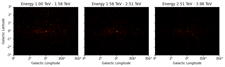
The same operation will be applied to all other maps contained in the datasets such as mask_fit:
[29]:
sliced.mask_fit.plot_grid();
Resampling datasets#
It can often be useful to coarsely rebin an initially computed datasets by a specified factor. This can be done in either spatial or energy axes:
[30]:
downsampled = dataset_cta.downsample(factor=8)
downsampled.counts.sum_over_axes().plot()
[30]:
<WCSAxesSubplot:xlabel='Galactic Longitude', ylabel='Galactic Latitude'>
And the same downsampling process is possible along the energy axis:
[31]:
downsampled_energy = dataset_cta.downsample(
    factor=5, axis_name="energy", name="downsampled-energy"
)
downsampled_energy.counts.plot_grid();
In the printout one can see that the actual number of counts is preserved during the downsampling:
[32]:
print(downsampled_energy, dataset_cta)
MapDataset
----------

  Name                            : downsampled-energy

  Total counts                    : 104317
  Total background counts         : 91507.69
  Total excess counts             : 12809.31

  Predicted counts                : 91507.69
  Predicted background counts     : 91507.69
  Predicted excess counts         : nan

  Exposure min                    : 6.28e+07 m2 s
  Exposure max                    : 1.90e+10 m2 s

  Number of total bins            : 153600
  Number of fit bins              : 22608

  Fit statistic type              : cash
  Fit statistic value (-2 log(L)) : nan

  Number of models                : 0
  Number of parameters            : 0
  Number of free parameters       : 0

 MapDataset
----------

  Name                            : dataset-cta

  Total counts                    : 104317
  Total background counts         : 91507.70
  Total excess counts             : 12809.30

  Predicted counts                : 91719.65
  Predicted background counts     : 91507.69
  Predicted excess counts         : 211.96

  Exposure min                    : 6.28e+07 m2 s
  Exposure max                    : 1.90e+10 m2 s

  Number of total bins            : 768000
  Number of fit bins              : 67824

  Fit statistic type              : cash
  Fit statistic value (-2 log(L)) : 44317.66

  Number of models                : 2
  Number of parameters            : 8
  Number of free parameters       : 5

  Component 0: SkyModel

    Name                      : gc
    Datasets names            : None
    Spectral model type       : PowerLawSpectralModel
    Spatial  model type       : PointSpatialModel
    Temporal model type       :
    Parameters:
      index                         :      2.000   +/-    0.00
      amplitude                     :   1.00e-12   +/- 0.0e+00 1 / (cm2 s TeV)
      reference             (frozen):      1.000       TeV
      lon_0                         :      4.650   +/-    0.00 rad
      lat_0                         :     -0.505   +/-    0.00 rad

  Component 1: FoVBackgroundModel

    Name                      : dataset-cta-bkg
    Datasets names            : ['dataset-cta']
    Spectral model type       : PowerLawNormSpectralModel
    Parameters:
      norm                          :      1.000   +/-    0.00
      tilt                  (frozen):      0.000
      reference             (frozen):      1.000       TeV
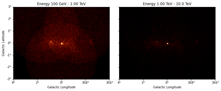
We can also resample the finer binned datasets to an arbitrary coarser energy binning using:
[33]:
energy_axis_new = MapAxis.from_energy_edges([0.1, 0.3, 1, 3, 10] * u.TeV)
resampled = dataset_cta.resample_energy_axis(energy_axis=energy_axis_new)
resampled.counts.plot_grid(ncols=2);
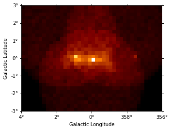
To squash the whole dataset into a single energy bin there is the .to_image() convenience method:
[34]:
dataset_image = dataset_cta.to_image()
dataset_image.counts.plot()
[34]:
<WCSAxesSubplot:xlabel='Galactic Longitude', ylabel='Galactic Latitude'>
SpectrumDataset#
SpectrumDataset inherits from a MapDataset, and is specially adapted for 1D spectral analysis, and uses a RegionGeom instead of a WcsGeom. A MapDatset can be converted to a SpectrumDataset, by summing the counts and background inside the on_region, which can then be used for classical spectral analysis. Containment correction is feasible only for circular regions.
[35]:
region = CircleSkyRegion(
    SkyCoord(0, 0, unit="deg", frame="galactic"), 0.5 * u.deg
)
spectrum_dataset = dataset_cta.to_spectrum_dataset(
    region, containment_correction=True, name="spectrum-dataset"
)
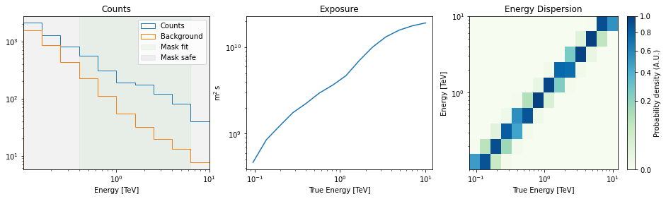
[36]:
# For a quick look
spectrum_dataset.peek();
A MapDataset can also be integrated over the on_region to create a MapDataset with a RegionGeom. Complex regions can be handled and since the full IRFs are used, containment correction is not required.
[37]:
reg_dataset = dataset_cta.to_region_map_dataset(
    region, name="region-map-dataset"
)
print(reg_dataset)
MapDataset
----------

  Name                            : region-map-dataset

  Total counts                    : 5644
  Total background counts         : 3323.66
  Total excess counts             : 2320.34

  Predicted counts                : 3323.66
  Predicted background counts     : 3323.66
  Predicted excess counts         : nan

  Exposure min                    : 4.66e+08 m2 s
  Exposure max                    : 1.89e+10 m2 s

  Number of total bins            : 10
  Number of fit bins              : 6

  Fit statistic type              : cash
  Fit statistic value (-2 log(L)) : nan

  Number of models                : 0
  Number of parameters            : 0
  Number of free parameters       : 0
FluxPointsDataset#
FluxPointsDataset is a Dataset container for precomputed flux points, which can be then used in fitting. FluxPointsDataset cannot be read directly, but should be read through FluxPoints, with an additional SkyModel. Similarly, FluxPointsDataset.write only saves the data component to disk.
[38]:
flux_points = FluxPoints.read(
    "$GAMMAPY_DATA/tests/spectrum/flux_points/diff_flux_points.fits"
)
model = SkyModel(spectral_model=PowerLawSpectralModel(index=2.3))
fp_dataset = FluxPointsDataset(data=flux_points, models=model)
No reference model set for FluxMaps. Assuming point source with E^-2 spectrum.
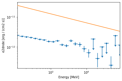
[39]:
fp_dataset.plot_spectrum()
[39]:
<AxesSubplot:xlabel='Energy [MeV]', ylabel='e2dnde [erg / (cm2 s)]'>
The masks on FluxPointsDataset are np.array and the data is a FluxPoints object. The mask_safe, by default, masks the upper limit points
[40]:
fp_dataset.mask_safe # Note: the mask here is simply a numpy array
[40]:
array([ True,  True,  True,  True,  True,  True,  True,  True,  True,
        True,  True,  True,  True,  True,  True,  True,  True, False,
        True, False, False,  True, False, False])
[41]:
fp_dataset.data # is a `FluxPoints` object
[41]:
<gammapy.estimators.points.core.FluxPoints at 0x16928c220>
[42]:
fp_dataset.data_shape() # number of data points
[42]:
(24,)
For an example of fitting FluxPoints, see flux point fitting, and can be used for catalog objects, eg see catalog notebook
Datasets#
Datasets are a collection of Dataset objects. They can be of the same type, or of different types, eg: mix of FluxPointDataset, MapDataset and SpectrumDataset.
For modelling and fitting of a list of Dataset objects, you can either - Do a joint fitting of all the datasets together - Stack the datasets together, and then fit them.
Datasets is a convenient tool to handle joint fitting of simultaneous datasets. As an example, please see the joint fitting tutorial
To see how stacking is performed, please see Implementation of stacking
To create a Datasets object, pass a list of Dataset on init, eg
[43]:
datasets = Datasets([dataset_empty, dataset_cta])
[44]:
print(datasets)
Datasets
--------

Dataset 0:

  Type       : MapDataset
  Name       : dataset-empty
  Instrument :
  Models     :

Dataset 1:

  Type       : MapDataset
  Name       : dataset-cta
  Instrument :
  Models     : ['gc', 'dataset-cta-bkg']
If all the datasets have the same type we can also print an info table, collectiong all the information from the individual casll to Dataset.info_dict():
[45]:
datasets.info_table() # quick info of all datasets
[45]:
| name | counts | excess | sqrt_ts | background | npred | npred_background | npred_signal | exposure_min | exposure_max | livetime | ontime | counts_rate | background_rate | excess_rate | n_bins | n_fit_bins | stat_type | stat_sum |
|---|---|---|---|---|---|---|---|---|---|---|---|---|---|---|---|---|---|---|
| m2 s | m2 s | s | s | 1 / s | 1 / s | 1 / s | ||||||||||||
| str13 | int64 | float64 | float64 | float64 | float64 | float64 | float64 | float64 | float64 | float64 | float64 | float64 | float64 | float64 | int64 | int64 | str4 | float64 |
| dataset-empty | 0 | 0.0 | 0.0 | 0.0 | 0.0 | 0.0 | nan | 0.0 | 0.0 | nan | 999.9999999999997 | nan | nan | nan | 110000 | 0 | cash | nan |
| dataset-cta | 104317 | 12809.3046875 | 41.41009347393684 | 91507.6953125 | 91719.64810194193 | 91507.68628538586 | 211.96181655608592 | 62842028.0 | 19024205824.0 | 5292.0001029780005 | 5400.0 | 19.712206721480793 | 17.291703237308198 | 2.4205034841725985 | 768000 | 67824 | cash | 44317.661091269125 |
[46]:
datasets.names # unique name of each dataset
[46]:
['dataset-empty', 'dataset-cta']
We can access individual datasets in Datasets object by name:
[47]:
datasets["dataset-empty"] # extracts the first dataset
[47]:
<gammapy.datasets.map.MapDataset at 0x1663fb130>
Or by index:
[48]:
datasets[0]
[48]:
<gammapy.datasets.map.MapDataset at 0x1663fb130>
Other list type operations work as well such as:
[49]:
# Use python list convention to remove/add datasets, eg:
datasets.remove("dataset-empty")
datasets.names
[49]:
['dataset-cta']
Or
[50]:
datasets.append(spectrum_dataset)
datasets.names
[50]:
['dataset-cta', 'spectrum-dataset']
Let’s create a list of spectrum datasets to illustrate some more functionality:
[51]:
datasets = Datasets()

path = make_path("$GAMMAPY_DATA/joint-crab/spectra/hess")

for filename in path.glob("pha_*.fits"):
    dataset = SpectrumDatasetOnOff.read(filename)
    datasets.append(dataset)
[52]:
print(datasets)
Datasets
--------

Dataset 0:

  Type       : SpectrumDatasetOnOff
  Name       : 23559
  Instrument :
  Models     :

Dataset 1:

  Type       : SpectrumDatasetOnOff
  Name       : 23523
  Instrument :
  Models     :

Dataset 2:

  Type       : SpectrumDatasetOnOff
  Name       : 23592
  Instrument :
  Models     :

Dataset 3:

  Type       : SpectrumDatasetOnOff
  Name       : 23526
  Instrument :
  Models     :
Now we can stack all datasets using .stack_reduce():
[53]:
stacked = datasets.stack_reduce(name="stacked")
print(stacked)
SpectrumDatasetOnOff
--------------------

  Name                            : stacked

  Total counts                    : 459
  Total background counts         : 27.50
  Total excess counts             : 431.50

  Predicted counts                : 45.27
  Predicted background counts     : 45.27
  Predicted excess counts         : nan

  Exposure min                    : 2.13e+06 m2 s
  Exposure max                    : 2.63e+09 m2 s

  Number of total bins            : 80
  Number of fit bins              : 43

  Fit statistic type              : wstat
  Fit statistic value (-2 log(L)) : 1530.36

  Number of models                : 0
  Number of parameters            : 0
  Number of free parameters       : 0

  Total counts_off                : 645
  Acceptance                      : 80
  Acceptance off                  : 2016
Or slice all datasets by a given energy range:
[54]:
datasets_sliced = datasets.slice_by_energy(
    energy_min="1 TeV", energy_max="10 TeV"
)
print(datasets_sliced.energy_ranges)
(<Quantity [1.e+09, 1.e+09, 1.e+09, 1.e+09] keV>, <Quantity [1.e+10, 1.e+10, 1.e+10, 1.e+10] keV>)