This is a fixed-text formatted version of a Jupyter notebook
Try online

You may download all the notebooks as a tar file.
Source files: cta_data_analysis.ipynb | cta_data_analysis.py
Basic image exploration and fitting#
Introduction#
This notebook shows an example how to make a sky image and spectrum for simulated CTA data with Gammapy.
The dataset we will use is three observation runs on the Galactic center. This is a tiny (and thus quick to process and play with and learn) subset of the simulated CTA dataset that was produced for the first data challenge in August 2017.
Setup#
As usual, we’ll start with some setup …
[1]:
%matplotlib inline
import matplotlib.pyplot as plt
[2]:
!gammapy info --no-envvar --no-system
Gammapy package:

        version                : 0.20
        path                   : /Users/adonath/github/adonath/gammapy/gammapy


WARNING: version mismatch between CFITSIO header (v4.000999999999999) and linked library (v4.01).


WARNING: version mismatch between CFITSIO header (v4.000999999999999) and linked library (v4.01).


WARNING: version mismatch between CFITSIO header (v4.000999999999999) and linked library (v4.01).


Other packages:

        numpy                  : 1.22.3
        scipy                  : 1.8.0
        astropy                : 5.0.4
        regions                : 0.5
        click                  : 8.1.3
        yaml                   : 6.0
        IPython                : 8.3.0
        jupyterlab             : 3.4.0
        matplotlib             : 3.5.2
        pandas                 : 1.4.2
        healpy                 : 1.15.2
        iminuit                : 2.11.2
        sherpa                 : not installed
        naima                  : 0.10.0
        emcee                  : 3.1.1
        corner                 : 2.2.1
[3]:
import numpy as np
import astropy.units as u
from astropy.coordinates import SkyCoord
from regions import CircleSkyRegion
from gammapy.modeling import Fit
from gammapy.data import DataStore
from gammapy.datasets import (
    Datasets,
    FluxPointsDataset,
    SpectrumDataset,
    MapDataset,
)
from gammapy.modeling.models import (
    PowerLawSpectralModel,
    SkyModel,
    GaussianSpatialModel,
)
from gammapy.maps import MapAxis, WcsGeom, RegionGeom
from gammapy.makers import (
    MapDatasetMaker,
    SafeMaskMaker,
    SpectrumDatasetMaker,
    ReflectedRegionsBackgroundMaker,
)
from gammapy.estimators import TSMapEstimator, FluxPointsEstimator
from gammapy.estimators.utils import find_peaks
from gammapy.visualization import plot_spectrum_datasets_off_regions
[4]:
# Configure the logger, so that the spectral analysis
# isn't so chatty about what it's doing.
import logging

logging.basicConfig()
log = logging.getLogger("gammapy.spectrum")
log.setLevel(logging.ERROR)
Select observations#
A Gammapy analysis usually starts by creating a gammapy.data.DataStore and selecting observations.
This is shown in detail in the other notebook, here we just pick three observations near the galactic center.
[5]:
data_store = DataStore.from_dir("$GAMMAPY_DATA/cta-1dc/index/gps")
[6]:
# Just as a reminder: this is how to select observations
# from astropy.coordinates import SkyCoord
# table = data_store.obs_table
# pos_obs = SkyCoord(table['GLON_PNT'], table['GLAT_PNT'], frame='galactic', unit='deg')
# pos_target = SkyCoord(0, 0, frame='galactic', unit='deg')
# offset = pos_target.separation(pos_obs).deg
# mask = (1 < offset) & (offset < 2)
# table = table[mask]
# table.show_in_browser(jsviewer=True)
[7]:
obs_id = [110380, 111140, 111159]
observations = data_store.get_observations(obs_id)
INFO:gammapy.data.data_store:Observations selected: 3 out of 3.
[8]:
obs_cols = ["OBS_ID", "GLON_PNT", "GLAT_PNT", "LIVETIME"]
data_store.obs_table.select_obs_id(obs_id)[obs_cols]
[8]:
| OBS_ID | GLON_PNT | GLAT_PNT | LIVETIME |
|---|---|---|---|
| deg | deg | s | |
| int64 | float64 | float64 | float64 |
| 110380 | 359.9999912037958 | -1.299995937905366 | 1764.0 |
| 111140 | 358.4999833830074 | 1.3000020211954284 | 1764.0 |
| 111159 | 1.5000056568267741 | 1.299940468335294 | 1764.0 |
Make sky images#
Define map geometry#
Select the target position and define an ON region for the spectral analysis
[9]:
axis = MapAxis.from_edges(
    np.logspace(-1.0, 1.0, 10), unit="TeV", name="energy", interp="log"
)
geom = WcsGeom.create(
    skydir=(0, 0), npix=(500, 400), binsz=0.02, frame="galactic", axes=[axis]
)
geom
[9]:
WcsGeom

        axes       : ['lon', 'lat', 'energy']
        shape      : (500, 400, 9)
        ndim       : 3
        frame      : galactic
        projection : CAR
        center     : 0.0 deg, 0.0 deg
        width      : 10.0 deg x 8.0 deg
        wcs ref    : 0.0 deg, 0.0 deg
Compute images#
[10]:
%%time
stacked = MapDataset.create(geom=geom)
stacked.edisp = None
maker = MapDatasetMaker(selection=["counts", "background", "exposure", "psf"])
maker_safe_mask = SafeMaskMaker(methods=["offset-max"], offset_max=2.5 * u.deg)

for obs in observations:
    cutout = stacked.cutout(obs.pointing_radec, width="5 deg")
    dataset = maker.run(cutout, obs)
    dataset = maker_safe_mask.run(dataset, obs)
    stacked.stack(dataset)
WARNING:gammapy.irf.background:Invalid unit found in background table! Assuming (s-1 MeV-1 sr-1)
WARNING:gammapy.irf.background:Invalid unit found in background table! Assuming (s-1 MeV-1 sr-1)
WARNING:gammapy.irf.background:Invalid unit found in background table! Assuming (s-1 MeV-1 sr-1)
CPU times: user 2.45 s, sys: 465 ms, total: 2.92 s
Wall time: 3.78 s
[11]:
# The maps are cubes, with an energy axis.
# Let's also make some images:
dataset_image = stacked.to_image()
Show images#
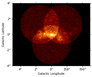
Let’s have a quick look at the images we computed …
[12]:
dataset_image.counts.smooth(2).plot(vmax=5);
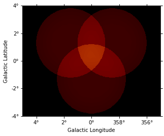
[13]:
dataset_image.background.plot(vmax=5);
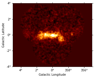
[14]:
dataset_image.excess.smooth(3).plot(vmax=2);
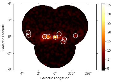
Source Detection#
Use the class gammapy.estimators.TSMapEstimator and function gammapy.estimators.utils.find_peaks to detect sources on the images. We search for 0.1 deg sigma gaussian sources in the dataset.
[15]:
spatial_model = GaussianSpatialModel(sigma="0.05 deg")
spectral_model = PowerLawSpectralModel(index=2)
model = SkyModel(spatial_model=spatial_model, spectral_model=spectral_model)
[16]:
ts_image_estimator = TSMapEstimator(
    model,
    kernel_width="0.5 deg",
    selection_optional=[],
    downsampling_factor=2,
    sum_over_energy_groups=False,
    energy_edges=[0.1, 10] * u.TeV,
)
[17]:
%%time
images_ts = ts_image_estimator.run(stacked)
CPU times: user 6.59 s, sys: 214 ms, total: 6.81 s
Wall time: 7.68 s
[18]:
sources = find_peaks(
    images_ts["sqrt_ts"],
    threshold=5,
    min_distance="0.2 deg",
)
sources
[18]:
| value | x | y | ra | dec |
|---|---|---|---|---|
| deg | deg | |||
| float64 | int64 | int64 | float64 | float64 |
| 35.937 | 252 | 197 | 266.42400 | -29.00490 |
| 17.899 | 207 | 202 | 266.85900 | -28.18386 |
| 12.762 | 186 | 200 | 267.14365 | -27.84496 |
| 9.9757 | 373 | 205 | 264.79470 | -30.97749 |
| 8.6616 | 306 | 185 | 266.01081 | -30.05120 |
| 8.0451 | 298 | 169 | 266.42267 | -30.08192 |
| 7.3817 | 274 | 217 | 265.77047 | -29.17056 |
| 6.692 | 90 | 209 | 268.07455 | -26.10409 |
| 5.0221 | 87 | 226 | 267.78333 | -25.87897 |
[19]:
source_pos = SkyCoord(sources["ra"], sources["dec"])
source_pos
[19]:
<SkyCoord (ICRS): (ra, dec) in deg
    [(266.42399798, -29.00490483), (266.85900392, -28.18385658),
     (267.14365055, -27.84495923), (264.79469899, -30.97749371),
     (266.01080642, -30.05120198), (266.4226731 , -30.08192101),
     (265.77046935, -29.1705559 ), (268.07454639, -26.10409446),
     (267.78332719, -25.87897418)]>
[20]:
# Plot sources on top of significance sky image
images_ts["sqrt_ts"].plot(add_cbar=True)

plt.gca().scatter(
    source_pos.ra.deg,
    source_pos.dec.deg,
    transform=plt.gca().get_transform("icrs"),
    color="none",
    edgecolor="white",
    marker="o",
    s=200,
    lw=1.5,
);
Spatial analysis#
See other notebooks for how to run a 3D cube or 2D image based analysis.
Spectrum#
We’ll run a spectral analysis using the classical reflected regions background estimation method, and using the on-off (often called WSTAT) likelihood function.
[21]:
target_position = SkyCoord(0, 0, unit="deg", frame="galactic")
on_radius = 0.2 * u.deg
on_region = CircleSkyRegion(center=target_position, radius=on_radius)
[22]:
exclusion_mask = ~geom.to_image().region_mask([on_region])
exclusion_mask.plot();
[23]:
energy_axis = MapAxis.from_energy_bounds(
    0.1, 40, 40, unit="TeV", name="energy"
)
energy_axis_true = MapAxis.from_energy_bounds(
    0.05, 100, 200, unit="TeV", name="energy_true"
)

geom = RegionGeom.create(region=on_region, axes=[energy_axis])
dataset_empty = SpectrumDataset.create(
    geom=geom, energy_axis_true=energy_axis_true
)
[24]:
dataset_maker = SpectrumDatasetMaker(
    containment_correction=False, selection=["counts", "exposure", "edisp"]
)
bkg_maker = ReflectedRegionsBackgroundMaker(exclusion_mask=exclusion_mask)
safe_mask_masker = SafeMaskMaker(methods=["aeff-max"], aeff_percent=10)
[25]:
%%time
datasets = Datasets()

for observation in observations:
    dataset = dataset_maker.run(
        dataset_empty.copy(name=f"obs-{observation.obs_id}"), observation
    )
    dataset_on_off = bkg_maker.run(dataset, observation)
    dataset_on_off = safe_mask_masker.run(dataset_on_off, observation)
    datasets.append(dataset_on_off)
CPU times: user 3.45 s, sys: 231 ms, total: 3.68 s
Wall time: 4.35 s
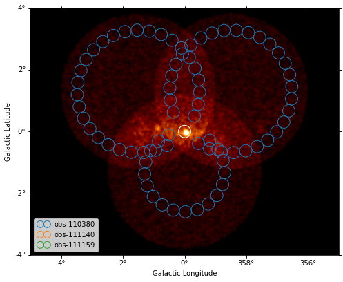
[26]:
plt.figure(figsize=(8, 8))
ax = dataset_image.counts.smooth("0.03 deg").plot(vmax=8)

on_region.to_pixel(ax.wcs).plot(ax=ax, edgecolor="white")
plot_spectrum_datasets_off_regions(datasets, ax=ax)
Model fit#
The next step is to fit a spectral model, using all data (i.e. a “global” fit, using all energies).
[27]:
%%time
spectral_model = PowerLawSpectralModel(
    index=2, amplitude=1e-11 * u.Unit("cm-2 s-1 TeV-1"), reference=1 * u.TeV
)

model = SkyModel(spectral_model=spectral_model, name="source-gc")

datasets.models = model

fit = Fit()
result = fit.run(datasets=datasets)
print(result)
OptimizeResult

        backend    : minuit
        method     : migrad
        success    : True
        message    : Optimization terminated successfully.
        nfev       : 104
        total stat : 88.36

CovarianceResult

        backend    : minuit
        method     : hesse
        success    : True
        message    : Hesse terminated successfully.

CPU times: user 1.27 s, sys: 17 ms, total: 1.29 s
Wall time: 1.57 s
Spectral points#
Finally, let’s compute spectral points. The method used is to first choose an energy binning, and then to do a 1-dim likelihood fit / profile to compute the flux and flux error.
[28]:
# Flux points are computed on stacked observation
stacked_dataset = datasets.stack_reduce(name="stacked")

print(stacked_dataset)
SpectrumDatasetOnOff
--------------------

  Name                            : stacked

  Total counts                    : 413
  Total background counts         : 85.43
  Total excess counts             : 327.57

  Predicted counts                : 98.34
  Predicted background counts     : 98.34
  Predicted excess counts         : nan

  Exposure min                    : 9.94e+07 m2 s
  Exposure max                    : 2.46e+10 m2 s

  Number of total bins            : 40
  Number of fit bins              : 30

  Fit statistic type              : wstat
  Fit statistic value (-2 log(L)) : 658.76

  Number of models                : 0
  Number of parameters            : 0
  Number of free parameters       : 0

  Total counts_off                : 2095
  Acceptance                      : 40
  Acceptance off                  : 990
[29]:
energy_edges = MapAxis.from_energy_bounds("1 TeV", "30 TeV", nbin=5).edges

stacked_dataset.models = model

fpe = FluxPointsEstimator(energy_edges=energy_edges, source="source-gc")
flux_points = fpe.run(datasets=[stacked_dataset])
flux_points.to_table(sed_type="dnde", formatted=True)
[29]:
| e_ref | e_min | e_max | dnde | dnde_err | ts | sqrt_ts | npred [1] | npred_excess [1] | stat | is_ul | counts [1] | success |
|---|---|---|---|---|---|---|---|---|---|---|---|---|
| TeV | TeV | TeV | 1 / (cm2 s TeV) | 1 / (cm2 s TeV) | ||||||||
| float64 | float64 | float64 | float64 | float64 | float64 | float64 | float64 | float32 | float64 | bool | float64 | bool |
| 1.375 | 0.946 | 2.000 | 1.447e-12 | 1.783e-13 | 152.513 | 12.350 | 105.77522448727254 | 83.89892 | 13.412 | False | 106.0 | True |
| 2.699 | 2.000 | 3.641 | 3.563e-13 | 4.835e-14 | 150.654 | 12.274 | 73.02511912207935 | 63.13247 | 2.245 | False | 73.0 | True |
| 5.295 | 3.641 | 7.700 | 7.332e-14 | 1.138e-14 | 121.570 | 11.026 | 53.983592085361686 | 47.455875 | 0.624 | False | 54.0 | True |
| 11.198 | 7.700 | 16.284 | 6.353e-15 | 2.154e-15 | 21.789 | 4.668 | 13.188429838184586 | 10.660447 | 5.744 | False | 13.0 | True |
| 21.971 | 16.284 | 29.645 | 1.109e-15 | 6.938e-16 | 6.250 | 2.500 | 4.1453105388557585 | 3.197989 | 2.899 | False | 4.0 | True |
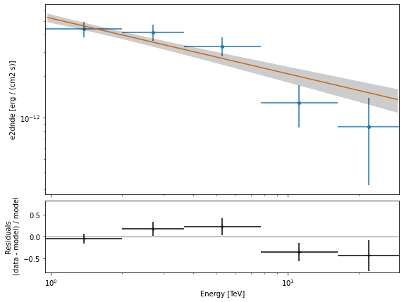
Plot#
Let’s plot the spectral model and points. You could do it directly, but for convenience we bundle the model and the flux points in a FluxPointDataset:
[30]:
flux_points_dataset = FluxPointsDataset(data=flux_points, models=model)
[31]:
flux_points_dataset.plot_fit();
Exercises#
Re-run the analysis above, varying some analysis parameters, e.g.
Select a few other observations
Change the energy band for the map
Change the spectral model for the fit
Change the energy binning for the spectral points
Change the target. Make a sky image and spectrum for your favourite source.
If you don’t know any, the Crab nebula is the “hello world!” analysis of gamma-ray astronomy.
[32]:
# print('hello world')
# SkyCoord.from_name('crab')
What next?#
This notebook showed an example of a first CTA analysis with Gammapy, using simulated 1DC data.
Let us know if you have any question or issues!