Constraining parameter limits

Explore how to deal with upper limits on parameters.

Prerequisites

It is advisable to understand the general Gammapy modelling and fitting framework before proceeding with this notebook, e.g. see Modeling and Fitting (DL4 to DL5).

Context

Even with significant detection of a source, constraining specific model parameters may remain difficult, allowing only for the calculation of confidence intervals.

Proposed approach

In this section, we will use 6 observations of the blazar PKS 2155-304, taken in 2008 by H.E.S.S, to constrain the curvature in the spectrum.

Setup

As usual, let’s start with some general imports…

# %matplotlib inline
import matplotlib.pyplot as plt

import numpy as np
import astropy.units as u
from gammapy.datasets import SpectrumDatasetOnOff, Datasets
from gammapy.modeling import Fit, select_nested_models
from gammapy.modeling.models import SkyModel, LogParabolaSpectralModel
from gammapy.estimators import FluxPointsEstimator

Load observation

We will use a SpectrumDatasetOnOff to see how to constrain model parameters. This dataset was obtained from H.E.S.S. observation of the blazar PKS 2155-304. Detailed modeling of this dataset can be found in the Account for spectral absorption due to the EBL notebook.

dataset_onoff = SpectrumDatasetOnOff.read(
    "$GAMMAPY_DATA/PKS2155-steady/pks2155-304_steady.fits.gz"
)
dataset_onoff.peek()
plt.show()

Fit spectrum

We will investigate the presence of spectral curvature by modeling the observed spectrum using a LogParabolaSpectralModel.

spectral_model = LogParabolaSpectralModel(
    amplitude="5e-12 TeV-1 s-1 cm-2", alpha=2, beta=0.5, reference=1.0 * u.TeV
)

model_pks = SkyModel(spectral_model, name="model_pks")
dataset_onoff.models = model_pks

fit = Fit()
result_pks = fit.run(dataset_onoff)
print(result_pks.models)

DatasetModels

Component 0: SkyModel

  Name                      : model_pks
  Datasets names            : None
  Spectral model type       : LogParabolaSpectralModel
  Spatial  model type       :
  Temporal model type       :
  Parameters:
    amplitude                     :   4.23e-12   +/- 9.5e-13 1 / (TeV s cm2)
    reference             (frozen):      1.000       TeV
    alpha                         :      3.351   +/-    0.35
    beta                          :      0.263   +/-    0.54

We see that the parameter beta (the curvature parameter) is poorly constrained as the errors are very large. Therefore, we will perform a likelihood ratio test to evaluate the significance of the curvature compared to the null hypothesis of no curvature. In the null hypothesis, beta=0.

LLR = select_nested_models(
    datasets=Datasets(dataset_onoff),
    parameters=[model_pks.parameters["beta"]],
    null_values=[0],
)
print(LLR)

{'ts': np.float64(0.32939559496572635), 'fit_results': <gammapy.modeling.fit.FitResult object at 0x7efd2222e3d0>, 'fit_results_null': <gammapy.modeling.fit.FitResult object at 0x7efd21d85910>}

We can see that the improvement in the test statistic after including the curvature is only ~0.3, which corresponds to a significance of only 0.5.

We can safely conclude that the addition of the curvature parameter does not significantly improve the fit. As a result, the function has internally updated the best fit model to the one corresponding to the null hypothesis (i.e. beta=0).

print(dataset_onoff.models)

DatasetModels

Component 0: SkyModel

  Name                      : model_pks
  Datasets names            : None
  Spectral model type       : LogParabolaSpectralModel
  Spatial  model type       :
  Temporal model type       :
  Parameters:
    amplitude                     :   3.85e-12   +/- 5.8e-13 1 / (TeV s cm2)
    reference             (frozen):      1.000       TeV
    alpha                         :      3.405   +/-    0.30
    beta                  (frozen):      0.000

Compute parameter asymmetric errors and upper limits

In such a case, it can still be useful to be able to constrain the allowed range of the non-significant parameter (e.g.: to rule out parameter values, to compare from theoretical predications, etc.).

First, we reset the alternative model on the dataset:

dataset_onoff.models = LLR["fit_results"].models
parameter = dataset_onoff.models.parameters["beta"]

We can then compute the asymmetric errors and upper limits on the parameter of interest. It is always useful to ensure that the fit the converged by looking at the success and message keywords.

res_1sig = fit.confidence(datasets=dataset_onoff, parameter=parameter, sigma=1)
print(res_1sig)

{'success': True, 'message': 'Minos terminated successfully.', 'errp': np.float64(0.8310464830801719), 'errn': np.float64(0.41346440407107254), 'nfev': 126}

We can directly use this to compute \(n\sigma\) upper limits on the parameter:

res_2sig = fit.confidence(datasets=dataset_onoff, parameter=parameter, sigma=2)
ll_2sigma = parameter.value - res_2sig["errn"]
ul_2sigma = parameter.value + res_2sig["errp"]

print(f"2-sigma lower limit on beta is {ll_2sigma:.2f}")
print(f"2-sigma upper limit on beta is {ul_2sigma:.2f}")

2-sigma lower limit on beta is -0.43
2-sigma upper limit on beta is 3.71

Likelihood profile

We can also compute the likelihood profile of the parameter. First we define the scan range such that it encompasses more than the 2-sigma parameter limits. Then we call stat_profile :

parameter.scan_n_values = 25
parameter.scan_min = parameter.value - 2.5 * res_2sig["errn"]
parameter.scan_max = parameter.value + 2.5 * res_2sig["errp"]
parameter.interp = "lin"
profile = fit.stat_profile(datasets=dataset_onoff, parameter=parameter, reoptimize=True)

The resulting profile is a dictionary that stores the likelihood value and the fit result for each value of beta.

print(profile)

{'model_pks.spectral.beta_scan': array([-1.4588051 , -1.02776659, -0.59672808, -0.16568956,  0.26534895,
        0.69638746,  1.12742597,  1.55846448,  1.98950299,  2.4205415 ,
        2.85158001,  3.28261852,  3.71365703,  4.14469554,  4.57573405,
        5.00677256,  5.43781107,  5.86884958,  6.29988809,  6.7309266 ,
        7.16196511,  7.59300362,  8.02404213,  8.45508064,  8.88611915]), 'stat_scan': array([50.67137298, 28.40382376, 13.59596178,  7.09723872,  6.00318251,
        6.40313003,  7.05413881,  7.6675433 ,  8.21483666,  8.71182744,
        9.17165555,  9.6013471 , 10.00441683, 10.38274403, 10.73753108,
       11.06974044, 11.38028286, 11.67009235, 11.94014857, 12.1914764 ,
       12.42513409, 12.64219749, 12.84374351, 13.03083462, 13.20450553]), 'fit_results': [<gammapy.modeling.fit.OptimizeResult object at 0x7efd2222edd0>, <gammapy.modeling.fit.OptimizeResult object at 0x7efd215bde10>, <gammapy.modeling.fit.OptimizeResult object at 0x7efd214f6d50>, <gammapy.modeling.fit.OptimizeResult object at 0x7efd21113c50>, <gammapy.modeling.fit.OptimizeResult object at 0x7efd1a098e90>, <gammapy.modeling.fit.OptimizeResult object at 0x7efd1bce7010>, <gammapy.modeling.fit.OptimizeResult object at 0x7efd21632e90>, <gammapy.modeling.fit.OptimizeResult object at 0x7efd21112190>, <gammapy.modeling.fit.OptimizeResult object at 0x7efd2a3eaf90>, <gammapy.modeling.fit.OptimizeResult object at 0x7efd1bc46e10>, <gammapy.modeling.fit.OptimizeResult object at 0x7efd222c6e50>, <gammapy.modeling.fit.OptimizeResult object at 0x7efd1a09b310>, <gammapy.modeling.fit.OptimizeResult object at 0x7efd2a3e9350>, <gammapy.modeling.fit.OptimizeResult object at 0x7efd21c0da50>, <gammapy.modeling.fit.OptimizeResult object at 0x7efd2295a990>, <gammapy.modeling.fit.OptimizeResult object at 0x7efd2195a810>, <gammapy.modeling.fit.OptimizeResult object at 0x7efd1bce4950>, <gammapy.modeling.fit.OptimizeResult object at 0x7efd22636510>, <gammapy.modeling.fit.OptimizeResult object at 0x7efd2a428190>, <gammapy.modeling.fit.OptimizeResult object at 0x7efd2195b690>, <gammapy.modeling.fit.OptimizeResult object at 0x7efd219f45d0>, <gammapy.modeling.fit.OptimizeResult object at 0x7efd219f6090>, <gammapy.modeling.fit.OptimizeResult object at 0x7efd2032b610>, <gammapy.modeling.fit.OptimizeResult object at 0x7efd1bb9d4d0>, <gammapy.modeling.fit.OptimizeResult object at 0x7efd2172ce10>]}

Let’s plot everything together

values = profile["model_pks.spectral.beta_scan"]
loglike = profile["stat_scan"]
ax = plt.gca()
ax.plot(values, loglike - np.min(loglike))
ax.set_xlabel("Beta")
ax.set_ylabel(r"$\Delta$TS")
ax.set_title(r"$\beta$-parameter likelihood profile")
ax.fill_betweenx(
    x1=parameter.value - res_2sig["errn"],
    x2=parameter.value + res_2sig["errp"],
    y=[-0.5, 25],
    alpha=0.3,
    color="pink",
    label="1-sigma range",
)
ax.fill_betweenx(
    x1=parameter.value - res_1sig["errn"],
    x2=parameter.value + res_1sig["errp"],
    y=[-0.5, 25],
    alpha=0.3,
    color="salmon",
    label="2-sigma range",
)
ax.set_ylim(-0.5, 25)
plt.legend()
plt.show()

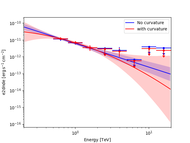
Impact of the model choice on the flux upper limits

The flux points depends on the underlying model assumption. This can have a non-negligible impact on the flux upper limits in the energy range where the model is not well constrained as illustrated in the following figure. So quote preferably upper limits from the model which is the most supported by the data.

energies = dataset_onoff.geoms["geom"].axes["energy"].edges
fpe = FluxPointsEstimator(energy_edges=energies, n_jobs=4, selection_optional=["ul"])

# Null hypothesis -- no curvature
dataset_onoff.models = LLR["fit_results_null"].models
fp_null = fpe.run(dataset_onoff)

# Alternative hypothesis -- with curvature
dataset_onoff.models = LLR["fit_results"].models
fp_alt = fpe.run(dataset_onoff)

Plot them together

ax = fp_null.plot(sed_type="e2dnde", color="blue")
LLR["fit_results_null"].models[0].spectral_model.plot(
    ax=ax,
    energy_bounds=(energies[0], energies[-1]),
    sed_type="e2dnde",
    color="blue",
    label="No curvature",
)
LLR["fit_results_null"].models[0].spectral_model.plot_error(
    ax=ax,
    energy_bounds=(energies[0], energies[-1]),
    sed_type="e2dnde",
    facecolor="blue",
    alpha=0.2,
)


fp_alt.plot(ax=ax, sed_type="e2dnde", color="red")
LLR["fit_results"].models[0].spectral_model.plot(
    ax=ax,
    energy_bounds=(energies[0], energies[-1]),
    sed_type="e2dnde",
    color="red",
    label="with curvature",
)
LLR["fit_results"].models[0].spectral_model.plot_error(
    ax=ax,
    energy_bounds=(energies[0], energies[-1]),
    sed_type="e2dnde",
    facecolor="red",
    alpha=0.2,
)

plt.legend()
plt.show()

This logic can be extended to any spectral or spatial feature. As an exercise, try to compute the 95% spatial extent on the MSH 15-52 dataset used for the ring background notebook.