Observational clustering

Clustering observations into specific groups.

Context

Typically, observations from gamma-ray telescopes can span a number of different observation periods, therefore it is likely that the observation conditions and quality are not always the same. This tutorial aims to provide a way in which observations can be grouped such that similar observations are grouped together, and then the data reduction is performed.

Objective

To cluster similar observations based on various quantities.

Proposed approach

For completeness two different methods for grouping of observations are shown here.

• A simple grouping based on zenith angle from an existing observations table.

• Grouping the observations depending on the IRF quality, by means of hierarchical clustering.

import numpy as np
import astropy.units as u
from astropy.coordinates import SkyCoord
import matplotlib.pyplot as plt
from gammapy.data import DataStore
from gammapy.data.utils import get_irfs_features
from gammapy.utils.cluster import hierarchical_clustering, standard_scaler

Obtain the observations

First need to define the DataStore object for the H.E.S.S. DL3 DR1 data. Next, utilise a cone search to select only the observations of interest. In this case, we choose PKS 2155-304 as the object of interest.

The ObservationTable is then filtered using the select_observations() tool.

data_store = DataStore.from_dir("$GAMMAPY_DATA/hess-dl3-dr1")

selection = dict(
    type="sky_circle",
    frame="icrs",
    lon="329.71693826 deg",
    lat="-30.2255 deg",
    radius="2 deg",
)
obs_table = data_store.obs_table
selected_obs_table = obs_table.select_observations(selection)

More complex selection can be done by utilising the obs_table entries directly. We can now retrieve the relevant observations by passing their obs_id to the get_observations method.

obs_ids = selected_obs_table["OBS_ID"]
observations = data_store.get_observations(obs_ids)

Show various observation quantities

Print here the range of zenith angles and muon efficiencies, to see if there is a sensible way to group the observations.

obs_zenith = selected_obs_table["ZEN_PNT"].to(u.deg)
obs_muoneff = selected_obs_table["MUONEFF"]

print(f"{np.min(obs_zenith):.2f} < zenith angle < {np.max(obs_zenith):.2f}")
print(f"{np.min(obs_muoneff):.2f} < muon efficiency < {np.max(obs_muoneff):.2f}")

7.23 deg < zenith angle < 50.42 deg
0.97 < muon efficiency < 1.03

Manual grouping of observations

Here we can plot the zenith angle vs muon efficiency of the observations. We decide to group the observations according to their zenith angle. This is done manually as per a user defined cut, in this case we take the median value of the zenith angles to define each observation group.

This type of grouping can be utilised according to different parameters i.e. zenith angle, muon efficiency, offset angle. The quantity chosen can therefore be adjusted according to each specific science case.

median_zenith = np.median(obs_zenith)

labels = []
for obs in observations:
    zenith = obs.get_pointing_altaz(time=obs.tmid).zen
    labels.append("low_zenith" if zenith < median_zenith else "high_zenith")
grouped_observations = observations.group_by_label(labels)

print(grouped_observations)

{'group_high_zenith': <gammapy.data.observations.Observations object at 0x7f908a9f77d0>, 'group_low_zenith': <gammapy.data.observations.Observations object at 0x7f9082a0b390>}

The results for each group of observations is shown visually below.

fix, ax = plt.subplots(1, 1, figsize=(7, 5))
for obs in grouped_observations["group_low_zenith"]:
    ax.plot(
        obs.get_pointing_altaz(time=obs.tmid).zen,
        obs.meta.optional["MUONEFF"],
        "d",
        color="red",
    )
for obs in grouped_observations["group_high_zenith"]:
    ax.plot(
        obs.get_pointing_altaz(time=obs.tmid).zen,
        obs.meta.optional["MUONEFF"],
        "o",
        color="blue",
    )
ax.set_ylabel("Muon efficiency")
ax.set_xlabel("Zenith angle (deg)")
ax.axvline(median_zenith.value, ls="--", color="black")
plt.show()

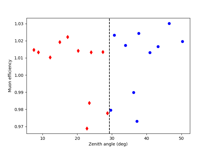
This shows the observations grouped by zenith angle. The diamonds are observations which have a zenith angle less than the median value, whilst the circles are observations above the median.

The grouped_observations provide a list of Observations which can be utilised in the usual way to show the various properties of the observations i.e. see the CTAO with Gammapy tutorial.

Hierarchical clustering of observations

This method shows how to cluster observations based on their IRF quantities, in this case those that have a similar edisp and psf. The get_irfs_features() is utilised to achieve this. The observations are then clustered based on these criteria using hierarchical_clustering. The idea here is to minimise the variance of both edisp and psf within a specific group to limit the error on the quantity when they are stacked at the dataset level.

In this example, the irf features are computed for the edisp-res and psf-radius at 1 TeV. This is stored as a Table, as shown below.

source_position = SkyCoord(329.71693826 * u.deg, -30.2255890 * u.deg, frame="icrs")
names = ["edisp-res", "psf-radius"]
features_irfs = get_irfs_features(
    observations, energy_true="1 TeV", position=source_position, names=names
)
print(features_irfs)

     edisp-res      obs_id      psf-radius
                                   deg
------------------- ------ -------------------
0.36834038301420274  33787 0.14149953611195087
 0.3398355551692374  33788 0.11553325504064559
 0.3237948926528733  33789 0.10262943822890519
 0.3053534585214654  33790 0.09426693227142095
0.28755283551094535  33791 0.08894569035619496
 0.2740949673532126  33792 0.08447355125099419
0.26665050077722524  33793  0.0811551760882139
 0.2627285490621433  33794 0.07943648658692837
0.26395547294386185  33795  0.0799109224230051
0.26887783978967333  33796 0.08191603310406206
 0.2777074437072966  33797  0.0855013383552432
 0.2935523826846635  33798  0.0897868126630783
 0.3118685761308288  33799 0.09623312838375568
0.33164865542240857  33800 0.10470702368766069
 0.3503706026275275  33801 0.12276676166802643
  0.301106169925983  47802 0.09740295372903346
 0.2861432787940169  47803 0.08880368117243051
0.27057337686547633  47804 0.08388624433428049
 0.2988221402797874  47827 0.09610314778983592
 0.2838535883996568  47828 0.08795162606984375
0.26866373287610784  47829 0.08328557573258877

Compute standardized features by removing the mean and scaling to unit variance:

scaled_features_irfs = standard_scaler(features_irfs)
print(scaled_features_irfs)

     edisp-res      obs_id       psf-radius
------------------- ------ ---------------------
  2.388594371509013  33787     3.053212009682775
  1.435163619575667  33788     1.363472509034498
 0.8986348249565016  33789    0.5237647004325865
  0.281804914378983  33790 -0.020420144596410953
-0.3135911172725387  33791  -0.36669663417038234
-0.7637304910949027  33792   -0.6577182894355391
-1.0127333408539105  33793    -0.873659477745188
-1.1439149565821138  33794    -0.985502122122975
-1.1028767519146723  33795   -0.9546285068162436
-0.9382332063153346  33796   -0.8241471833009617
-0.6429002210315774  33797    -0.590835686434463
-0.1129179960662306  33798   -0.3119611261122878
 0.4997228584905691  33799   0.10752883769757363
 1.1613278320355356  33800    0.6589622747787678
 1.7875403564022012  33801    1.8341884287660133
0.13974141617813501  47802    0.1836544903987521
-0.3607380331501994  47803   -0.3759377929871826
-0.8815208066507546  47804   -0.6959369197218669
 0.0633450907958376  47827   0.09907043184188653
-0.4373236994893457  47828   -0.4313847458879893
-0.9453946639008759  47829   -0.7350250533013533

The hierarchical_clustering then clusters this table into t=2 groups with a corresponding label for each group. In this case, we choose to cluster the observations into two groups. We can print this table to show the corresponding label which has been added to the previous feature_irfs table.

The arguments for fcluster are passed as a dictionary here.

features = hierarchical_clustering(scaled_features_irfs, fcluster_kwargs={"t": 2})
print(features)

     edisp-res      obs_id       psf-radius      labels
------------------- ------ --------------------- ------
  2.388594371509013  33787     3.053212009682775      1
  1.435163619575667  33788     1.363472509034498      1
 0.8986348249565016  33789    0.5237647004325865      1
  0.281804914378983  33790 -0.020420144596410953      2
-0.3135911172725387  33791  -0.36669663417038234      2
-0.7637304910949027  33792   -0.6577182894355391      2
-1.0127333408539105  33793    -0.873659477745188      2
-1.1439149565821138  33794    -0.985502122122975      2
-1.1028767519146723  33795   -0.9546285068162436      2
-0.9382332063153346  33796   -0.8241471833009617      2
-0.6429002210315774  33797    -0.590835686434463      2
-0.1129179960662306  33798   -0.3119611261122878      2
 0.4997228584905691  33799   0.10752883769757363      2
 1.1613278320355356  33800    0.6589622747787678      1
 1.7875403564022012  33801    1.8341884287660133      1
0.13974141617813501  47802    0.1836544903987521      2
-0.3607380331501994  47803   -0.3759377929871826      2
-0.8815208066507546  47804   -0.6959369197218669      2
 0.0633450907958376  47827   0.09907043184188653      2
-0.4373236994893457  47828   -0.4313847458879893      2
-0.9453946639008759  47829   -0.7350250533013533      2

Finally, observations.group_by_label creates a dictionary containing t Observations objects by grouping the similar labels.

obs_clusters = observations.group_by_label(features["labels"])
print(obs_clusters)


mask_1 = features["labels"] == 1
mask_2 = features["labels"] == 2
fix, ax = plt.subplots(1, 1, figsize=(7, 5))
ax.set_ylabel("edisp-res")
ax.set_xlabel("psf-radius")
ax.plot(
    features_irfs[mask_1]["edisp-res"],
    features_irfs[mask_1]["psf-radius"],
    "d",
    color="green",
    label="Group 1",
)
ax.plot(
    features_irfs[mask_2]["edisp-res"],
    features_irfs[mask_2]["psf-radius"],
    "o",
    color="magenta",
    label="Group 2",
)
ax.legend()
plt.show()

{'group_1': <gammapy.data.observations.Observations object at 0x7f9088e1c4d0>, 'group_2': <gammapy.data.observations.Observations object at 0x7f9088e1c090>}

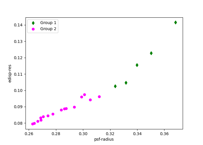
The groups here are divided by the quality of the IRFs values edisp-res and psf-radius. The diamond and circular points indicate how the observations are grouped.

In both examples we have a set of Observation objects which can be reduced using the DatasetsMaker to create two (in this specific case) separate datasets. These can then be jointly fitted using the Multi instrument joint 3D and 1D analysis tutorial.