Make a theta-square plot

This tutorial explains how to make such a plot, that is the distribution of event counts as a function of the squared angular distance, to a test position.

Setup

# %matplotlib inline
import matplotlib.pyplot as plt
from astropy.coordinates import SkyCoord
from astropy import units as u
from gammapy.data import DataStore
from gammapy.maps import MapAxis
from gammapy.makers.utils import ThetaSquaredTable
from gammapy.visualization import plot_theta_squared_table

Get some data

Some data taken on the Crab by H.E.S.S. are used.

data_store = DataStore.from_dir("$GAMMAPY_DATA/hess-dl3-dr1")
observations = data_store.get_observations([23523, 23526])

Define a test position

Here we define the position of Crab

position = SkyCoord(83.6324, 22.0174, unit="deg")
print(position)

<SkyCoord (ICRS): (ra, dec) in deg
    (83.6324, 22.0174)>

Creation of the theta2 plot

By default, the distribution of the OFF counts in squared angular distance is calculated from the mirror reflected coordinates of the test position, assuming therefore a single OFF position. However, one can set manually both the coordinates of the off_position. It is worth to note that overlapping regions are always forbidden to avoid correlated OFF counts, therefore the user should take care in the choice of the off_position.

separation = position.separation(observations[0].pointing.fixed_icrs)
position_angle = 180 * u.deg
off_position = position.directional_offset_by(
    position_angle=position_angle, separation=separation * 2
)
print(off_position)

<SkyCoord (ICRS): (ra, dec) in deg
    (83.6324, 21.0114874)>

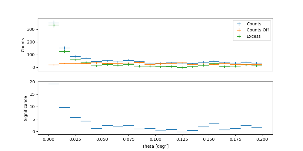
theta2_axis = MapAxis.from_bounds(0, 0.2, nbin=20, interp="lin", unit="deg2")
theta2_table_maker = ThetaSquaredTable(
    observations=observations,
    position=position,
    theta_squared_axis=theta2_axis,
    position_off=off_position,
)
theta2_table = theta2_table_maker.run()

plt.figure(figsize=(10, 5))
plot_theta_squared_table(theta2_table)
plt.show()

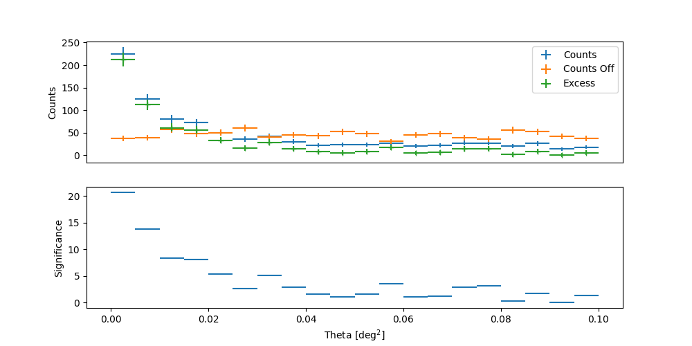
Alternatively, it can be requested a number of reflected OFF positions that will be calculated through the WobbleRegionsFinder. As mentioned before, the user should be cautious that the regions (ON and OFF) do not overlap, otherwise only the mirror reflected region will be adopted as OFF.

off_regions_number = 3
theta2_axis = MapAxis.from_bounds(0, 0.1, nbin=20, interp="lin", unit="deg2")
theta2_table_maker_offreg = ThetaSquaredTable(
    observations=observations,
    position=position,
    theta_squared_axis=theta2_axis,
    off_regions_number=off_regions_number,
)
theta2_table_offreg = theta2_table_maker_offreg.run()

plt.figure(figsize=(10, 5))
plot_theta_squared_table(theta2_table_offreg)
plt.show()

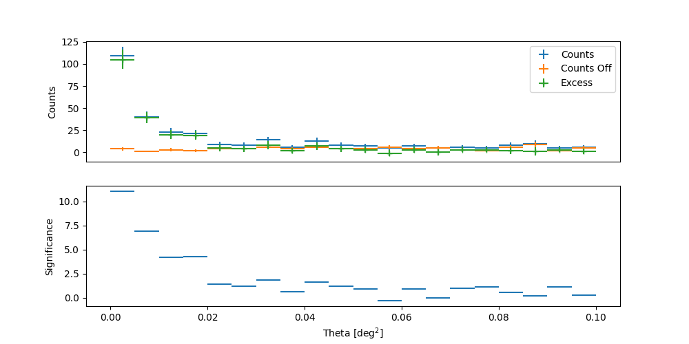
Making a theta2 plot for a given energy range

With the function ThetaSquaredTable, one can also select a fixed energy range.

theta2_table_maker_en = ThetaSquaredTable(
    observations=observations,
    position=position,
    theta_squared_axis=theta2_axis,
    energy_edges=[1.2, 11] * u.TeV,
)
theta2_table_en = theta2_table_maker_en.run()

plt.figure(figsize=(10, 5))
plot_theta_squared_table(theta2_table_en)
plt.show()

Statistical significance of a detection

To get the significance of a signal, the usual method consists of using the reflected background method (see the maker tutorial: Reflected regions background) to compute the WStat statistics (see WStat : Poisson data with background measurement, Fit statistics). This is the well-known method of [LiMa1983] using ON and OFF regions.

The following tutorials show how to get an excess significance:

• Spectral analysis

• Spectral analysis of extended sources