This is a fixed-text formatted version of a Jupyter notebook.

Try online
You can contribute with your own notebooks in this GitHub repository.
Source files: source_population_model.ipynb | source_population_model.py

Astrophysical source population modeling with Gammapy¶

Introduction¶

The gammapy.astro.population package contains some simple Galactic source population models.

Here we provide some Python code to compute observable parameter distributions for Galactic gamma-ray source populations.

Observables: Flux, GLON, GLAT
Source classes: Pulsar (PSR), Supernova remnant (SNR), pulsar wind nebula (PWN)

References:

Section 6.2 in the Fermi-LAT collaboration paper “The First Fermi-LAT Catalog of Sources Above 10 GeV”
Axel Donath’s bachelor thesis “Modelling Galactic gamma-ray source populations”, specifically Chapter 4.
Casanova & Dingus (2008), “Constraints on the TeV source population and its contribution to the galactic diffuse TeV emission”
Strong (2007), “Source population synthesis and the Galactic diffuse gamma-ray emission”

Setup¶

In [1]:

%matplotlib inline
import matplotlib.pyplot as plt

In [2]:

import numpy as np
import astropy.units as u
from gammapy.utils.random import sample_powerlaw
from gammapy.astro import population

Simulate positions¶

In [3]:

# Spatial distribution using Lorimer (2006) model
n_sources = int(1e5)

table = population.make_base_catalog_galactic(
    n_sources=n_sources,
    rad_dis="L06",
    vel_dis="F06B",
    max_age=1e6 * u.yr,
    spiralarms=True,
)

Simulate luminosities¶

Several source population models, e.g. the 1FHL paper or Strong (2007), use power-law luminosity functions.

Here we implement the “reference model” from the 1FHL catalog paper section 6.2.

In [4]:

# Source luminosity (ph s^-1)

luminosity = sample_powerlaw(x_min=1e34, x_max=1e37, gamma=1.5, size=n_sources)
table["luminosity"] = luminosity

Compute observable parameters¶

In [5]:

table = population.add_observed_parameters(table)
table.info()

<Table length=100000>
   name     dtype     unit                description
---------- ------- --------- --------------------------------------
       age float64        yr                      Age of the source
     n_ISM float64   1 / cm3            Interstellar medium density
 spiralarm   str18                                 Which spiralarm?
   x_birth float64       kpc   Galactocentric x coordinate at birth
   y_birth float64       kpc   Galactocentric y coordinate at birth
   z_birth float64       kpc   Galactocentric z coordinate at birth
         x float64       kpc            Galactocentric x coordinate
         y float64       kpc            Galactocentric y coordinate
         z float64       kpc            Galactocentric z coordinate
        vx float64    km / s Galactocentric velocity in x direction
        vy float64    km / s Galactocentric velocity in y direction
        vz float64    km / s Galactocentric velocity in z direction
     v_abs float64    km / s     Galactocentric velocity (absolute)
luminosity float64
  distance float64        pc     Distance observer to source center
      GLON float64       deg                     Galactic longitude
      GLAT float64       deg                      Galactic latitude
     VGLON float64 deg / Myr         Velocity in Galactic longitude
     VGLAT float64 deg / Myr          Velocity in Galactic latitude
        RA float64       deg                        Right ascension
       DEC float64       deg                            Declination
      flux float64  1 / kpc2                            Source flux

Check output¶

The simulation is done, you could save the simulated catalog to a file.

Here we just plot a few distributions to check if the results look OK.

In [6]:

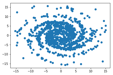
plt.scatter(table["x"][:1000], table["y"][:1000]);

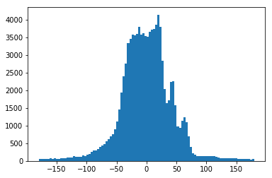
../_images/notebooks_source_population_model_15_0.png

In [7]:

plt.hist(table["GLON"], bins=100);

../_images/notebooks_source_population_model_16_0.png

In [8]:

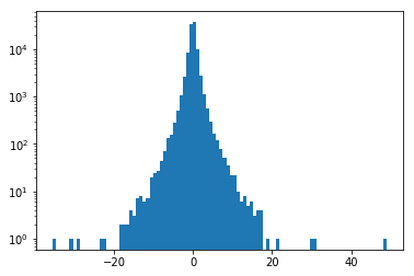
plt.hist(table["GLAT"], bins=100, log=True);

../_images/notebooks_source_population_model_17_0.png

In [9]:

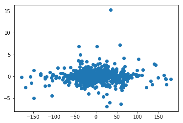
plt.scatter(table["GLON"][:1000], table["GLAT"][:1000]);

../_images/notebooks_source_population_model_18_0.png

In [10]:

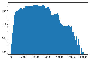
plt.hist(table["distance"], bins=100, log=True);

../_images/notebooks_source_population_model_19_0.png

In [11]:

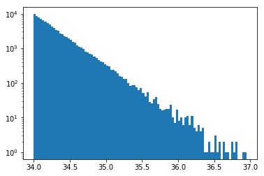
plt.hist(np.log10(table["luminosity"]), bins=100, log=True);

../_images/notebooks_source_population_model_20_0.png

In [12]:

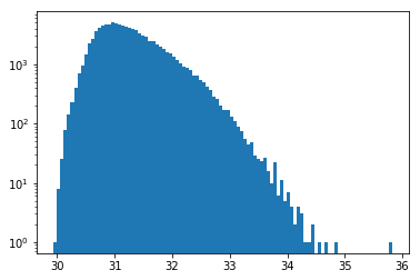
plt.hist(np.log10(table["flux"]), bins=100, log=True);

../_images/notebooks_source_population_model_21_0.png

In [13]:

# TODO: plot GLON, GLAT, FLUX distribution

Exercises¶

TODO

In [14]:

# Start exercises here

What next?¶

TODO: summarise what was done here briefly.

TODO: add some pointers to other documentation.