This is a fixed-text formatted version of a Jupyter notebook.
- Try online

- You can contribute with your own notebooks in this GitHub repository.
- Source files: hgps.ipynb | hgps.py
HGPS
Introduction
The H.E.S.S. Galactic Plane Survey (HGPS) is the first deep and wide survey of the Milky Way in TeV gamma-rays.
In April 2018, a paper on the HGPS was published, and survey maps and a source catalog on the HGPS in FITS format released.
More information, and the HGPS data for download in FITS format is available here: https://www.mpi-hd.mpg.de/hfm/HESS/hgps
Please read the Appendix A of the paper to learn about the caveats to using the HGPS data. Especially note that the HGPS survey maps are correlated and thus no detailed source morphology analysis is possible, and also note the caveats concerning spectral models and spectral flux points.
Notebook Overview
This is a Jupyter notebook that illustrates how to work with the HGPS data from Python.
You will learn how to access the HGPS images as well as the HGPS catalog and other tabular data using Astropy and Gammapy.
- In the first part we will only use Astropy to do some basic things.
- Then in the second part we’ll use Gammapy to do some things that are a little more advanced.
The notebook is pretty long: feel free to skip ahead to a section of your choice after executing the cells in the “Setup” and “Download data” sections below.
Note that there are other tools to work with FITS data that we don’t explain here. Specifically DS9 and Aladin are good FITS image viewers, and TOPCAT is great for FITS tables. Astropy and Gammapy are just one way to work with the HGPS data; any tool that can access FITS data can be used.
Packages
We will be using the following Python packages
- astropy
- gammapy
- matplotlib for plotting
Under the hood all of those packages use Numpy arrays to store and work with data.
More specifically, we will use the following functions and classes:
- From astropy, we will use astropy.io.fits to read the FITS data, astropy.table.Table to work with the tables, but also astropy.coordinates.SkyCoord and astropy.wcs.WCS to work with sky and pixel coordinates and astropy.units.Quantity to work with quantities.
- From gammapy, we will use gammapy.maps.WcsNDMap to work with the HGPS sky maps, and gammapy.catalog.SourceCatalogHGPS and gammapy.catalog.SourceCatalogObjectHGPS to work with the HGPS catalog data, especially the HGPS spectral data using gammapy.spectrum.models.SpectralModel and gammapy.spectrum.FluxPoints objects.
- matplotlib for all plotting. For sky image plotting, we will use matplotlib via astropy.visualization and gammapy.maps.WcsNDMap.plot.
If you’re not familiar with Python, Numpy, Astropy, Gammapy or matplotlib yet, use the tutorial introductions as explained here, as well as the links to the documentation that we just mentioned.
Setup
We start by importing everything we will use in this notebook, and configuring the notebook to show plots inline.
If you get an error here, you probably have to install the missing package and re-start the notebook.
If you don’t get an error, just go ahead, no nead to read the import code and text in this section.
In [1]:
import numpy as np
In [2]:
import astropy.units as u
from astropy.coordinates import SkyCoord
from astropy.io import fits
from astropy.table import Table
from astropy.wcs import WCS

import astropy

print(astropy.__version__)
3.0.5
In [3]:
from gammapy.maps import Map
from gammapy.catalog import SourceCatalogHGPS

import gammapy

print(gammapy.__version__)
0.9
In [4]:
%matplotlib inline
import matplotlib.pyplot as plt

import matplotlib

print(matplotlib.__version__)
3.0.2
In [5]:
# This will work on Python 2 as well as Python 3
from gammapy.extern.six.moves.urllib.request import urlretrieve
from gammapy.extern.pathlib import Path
Download Data
First, you need to download the HGPS FITS data from https://www.mpi-hd.mpg.de/hfm/HESS/hgps .
If you haven’t already, you can use the following commands to download the files to your local working directory.
You don’t have to read the code in the next cell; that’s just how to downlaod files from Python. You could also download the files with your web browser, or from the command line e.g. with curl:
mkdir hgps_data
cd hgps_data
curl -O https://www.mpi-hd.mpg.de/hfm/HESS/hgps/data/hgps_catalog_v1.fits.gz
curl -O https://www.mpi-hd.mpg.de/hfm/HESS/hgps/data/hgps_map_significance_0.1deg_v1.fits.gz
The rest of this notebook assumes that you have the data files at ``hgps_data_path``.
In [6]:
# Download HGPS data used in this tutorial to a folder of your choice
# The default `hgps_data` used here is a sub-folder in your current
# working directory (where you started the notebook)
hgps_data_path = Path("hgps_data")

# In this notebook we will only be working with the following files
# so we only download what is needed.
hgps_filenames = [
    "hgps_catalog_v1.fits.gz",
    "hgps_map_significance_0.1deg_v1.fits.gz",
]
In [7]:
def hgps_data_download():
    base_url = "https://www.mpi-hd.mpg.de/hfm/HESS/hgps/data/"
    for filename in hgps_filenames:
        url = base_url + filename
        path = hgps_data_path / filename
        if path.exists():
            print("Already downloaded: {}".format(path))
        else:
            print("Downloading {} to {}".format(url, path))
            urlretrieve(url, str(path))


hgps_data_path.mkdir(parents=True, exist_ok=True)
hgps_data_download()

print("\n\nFiles at {} :\n".format(hgps_data_path.absolute()))
for path in hgps_data_path.iterdir():
    print(path)
Downloading https://www.mpi-hd.mpg.de/hfm/HESS/hgps/data/hgps_catalog_v1.fits.gz to hgps_data/hgps_catalog_v1.fits.gz
Downloading https://www.mpi-hd.mpg.de/hfm/HESS/hgps/data/hgps_map_significance_0.1deg_v1.fits.gz to hgps_data/hgps_map_significance_0.1deg_v1.fits.gz


Files at /Users/deil/work/code/gammapy-docs/build/dev/gammapy/temp/hgps_data :

hgps_data/hgps_map_significance_0.1deg_v1.fits.gz
hgps_data/hgps_catalog_v1.fits.gz
Catalog with Astropy
FITS file content
Let’s start by just opening up hgps_catalog_v1.fits.gz and looking
at the content.
Note that astropy.io.fits.open doesn’t work with Path objects
yet, so you have to call str(path) and pass a string.
In [8]:
path = hgps_data_path / "hgps_catalog_v1.fits.gz"
hdu_list = fits.open(str(path))
In [9]:
hdu_list.info()
Filename: hgps_data/hgps_catalog_v1.fits.gz
No.    Name      Ver    Type      Cards   Dimensions   Format
  0  PRIMARY       1 PrimaryHDU      15   ()
  1  HGPS_SOURCES    1 BinTableHDU    327   78R x 78C   [16A, 6A, 10A, 20A, 7A, E, E, E, E, E, E, E, E, K, 18A, 103A, E, E, E, E, E, E, E, E, E, E, E, E, E, E, E, E, E, E, E, E, E, E, E, E, E, E, E, 4A, E, E, E, E, E, E, E, E, E, E, E, E, E, E, E, E, E, E, E, E, E, E, E, E, E, K, 40E, 40E, 40E, 40E, 40E, 40E, 40E, 40B]
  2  HGPS_GAUSS_COMPONENTS    1 BinTableHDU     87   98R x 13C   [9A, 16A, 15A, E, E, E, E, E, E, E, E, E, E]
  3  HGPS_ASSOCIATIONS    1 BinTableHDU     39   223R x 4C   [16A, 5A, 21A, E]
  4  HGPS_IDENTIFICATIONS    1 BinTableHDU     53   31R x 9C   [16A, 17A, 9A, 11A, 21A, 21A, E, E, E]
  5  HGPS_LARGE_SCALE_COMPONENT    1 BinTableHDU     55   50R x 7C   [E, E, E, E, E, E, E]
  6  SNRCAT        1 BinTableHDU     56   282R x 7C   [11A, E, E, 29A, E, E, E]
There are six tables. Each table and column is described in detail in the HGPS paper.
Access table data
We could work with the astropy.io.fits.HDUList and
astropy.io.fits.BinTable objects. However, in Astropy a nicer class
to work with tables has been developed: astropy.table.Table.
We will only be using Table, so let’s convert the FITS tabular data
into a Table object:
In [10]:
table = Table.read(hdu_list["HGPS_SOURCES"])

# Alternatively, reading from file directly would work like this:
# table = Table.read(str(path), hdu='HGPS_SOURCES')
# Usually you have to look first what HDUs are in a FITS file
# like we did above; `Table` is just for one table
In [11]:
# List available columns
table.info()
# To get shorter output here, we just list a few
# table.info(out=None)['name', 'dtype', 'shape', 'unit'][:10]
<Table length=78>
             name               dtype  shape       unit      n_bad
------------------------------ ------- ----- --------------- -----
                   Source_Name   str16                           0
            Analysis_Reference    str6                           0
                  Source_Class   str10                           0
             Identified_Object   str20                           0
           Gamma_Cat_Source_ID    str7                           0
                       RAJ2000 float32                   deg     0
                       DEJ2000 float32                   deg     0
                          GLON float32                   deg     0
                      GLON_Err float32                   deg    14
                          GLAT float32                   deg     0
                      GLAT_Err float32                   deg    14
                    Pos_Err_68 float32                   deg     3
                    Pos_Err_95 float32                   deg    14
                    ROI_Number   int64                           0
                 Spatial_Model   str18                           0
                    Components  str103                           0
                       Sqrt_TS float32                          14
                          Size float32                   deg    23
                      Size_Err float32                   deg    25
                       Size_UL float32                   deg    61
                           R70 float32                   deg    14
                         RSpec float32                   deg     0
            Excess_Model_Total float32                          14
                  Excess_RSpec float32                          14
            Excess_RSpec_Model float32                          14
              Background_RSpec float32                          14
                      Livetime float32                     h     0
              Energy_Threshold float32                   TeV    14
                      Flux_Map float32           1 / (cm2 s)     0
                  Flux_Map_Err float32           1 / (cm2 s)     0
           Flux_Map_RSpec_Data float32           1 / (cm2 s)    14
         Flux_Map_RSpec_Source float32           1 / (cm2 s)    14
          Flux_Map_RSpec_Other float32           1 / (cm2 s)    14
             Flux_Map_RSpec_LS float32           1 / (cm2 s)    14
          Flux_Map_RSpec_Total float32           1 / (cm2 s)    14
             Containment_RSpec float32                          14
           Contamination_RSpec float32                          14
Flux_Correction_RSpec_To_Total float32                          14
                 Livetime_Spec float32                     h     0
         Energy_Range_Spec_Min float32                   TeV     1
         Energy_Range_Spec_Max float32                   TeV     5
               Background_Spec float32                          14
                   Excess_Spec float32                          14
                Spectral_Model    str4                           0
               TS_ECPL_over_PL float32                          70
            Flux_Spec_Int_1TeV float32           1 / (cm2 s)     0
        Flux_Spec_Int_1TeV_Err float32           1 / (cm2 s)     0
     Flux_Spec_Energy_1_10_TeV float32         erg / (cm2 s)     0
 Flux_Spec_Energy_1_10_TeV_Err float32         erg / (cm2 s)     0
          Energy_Spec_PL_Pivot float32                   TeV     4
       Flux_Spec_PL_Diff_Pivot float32       1 / (cm2 s TeV)     4
   Flux_Spec_PL_Diff_Pivot_Err float32       1 / (cm2 s TeV)     4
        Flux_Spec_PL_Diff_1TeV float32       1 / (cm2 s TeV)     4
    Flux_Spec_PL_Diff_1TeV_Err float32       1 / (cm2 s TeV)     4
                 Index_Spec_PL float32                           4
             Index_Spec_PL_Err float32                           4
        Energy_Spec_ECPL_Pivot float32                   TeV    66
     Flux_Spec_ECPL_Diff_Pivot float32       1 / (cm2 s TeV)    66
 Flux_Spec_ECPL_Diff_Pivot_Err float32       1 / (cm2 s TeV)    66
      Flux_Spec_ECPL_Diff_1TeV float32       1 / (cm2 s TeV)    66
  Flux_Spec_ECPL_Diff_1TeV_Err float32       1 / (cm2 s TeV)    66
               Index_Spec_ECPL float32                          66
           Index_Spec_ECPL_Err float32                          66
              Lambda_Spec_ECPL float32               1 / TeV    66
          Lambda_Spec_ECPL_Err float32               1 / TeV    66
         Flux_Spec_PL_Int_1TeV float32           1 / (cm2 s)     4
     Flux_Spec_PL_Int_1TeV_Err float32           1 / (cm2 s)     4
       Flux_Spec_ECPL_Int_1TeV float32           1 / (cm2 s)    66
   Flux_Spec_ECPL_Int_1TeV_Err float32           1 / (cm2 s)    66
                 N_Flux_Points   int64                           0
            Flux_Points_Energy float32 (40,)             TeV  2546
        Flux_Points_Energy_Min float32 (40,)             TeV  2647
        Flux_Points_Energy_Max float32 (40,)             TeV  2647
              Flux_Points_Flux float32 (40,) 1 / (cm2 s TeV)  2558
       Flux_Points_Flux_Err_Lo float32 (40,) 1 / (cm2 s TeV)  2558
       Flux_Points_Flux_Err_Hi float32 (40,) 1 / (cm2 s TeV)  2558
           Flux_Points_Flux_UL float32 (40,) 1 / (cm2 s TeV)  2724
        Flux_Points_Flux_Is_UL   uint8 (40,)                     0
In [12]:
# Rows are accessed by indexing into the table
# with an integer index (Python starts at index 0)
# table[0]
# To get shorter output here, we just list a few
table[table.colnames[:5]][0]
Out[12]:
| Source_Name | Analysis_Reference | Source_Class | Identified_Object | Gamma_Cat_Source_ID |
|---|---|---|---|---|
| str16 | str6 | str10 | str20 | str7 |
| HESS J0835-455 | HGPS | PWN | Vela X | 37 |
In [13]:
# Columns are accessed by indexing into the table
# with a column name string
# Then you can slice the column to get the rows you want
table["Source_Name"][:5]
Out[13]:
| HESS J0835-455 |
| HESS J0852-463 |
| HESS J1018-589 A |
| HESS J1018-589 B |
| HESS J1023-575 |
In [14]:
# Accessing a given element of the table like this
table["Source_Name"][5]
Out[14]:
'HESS J1026-582'
In [15]:
# If you know some Python and Numpy, you can now start
# to ask questions about the HGPS data.
# Just to give one example: "What spatial models are used?"
In [16]:
set(table["Spatial_Model"])
Out[16]:
{'2-Gaussian', '3-Gaussian', 'Gaussian', 'Point-Like', 'Shell'}
Convert formats
The HGPS catalog is only released in FITS format.
We didn’t provide multiple formats (DS9, CSV, XML, VOTABLE, …) because everyone needs something a little different (in terms of format or content). Instead, here we show how you can convert to any format / content you like wiht a few lines of Python.
DS9 region format
At Fermi-LAT 3FGL webpage, we see that they also provide DS9 region files that look like this:
global color=red
fk5;point(   0.0377, 65.7517)# point=cross text={3FGL J0000.1+6545}
fk5;point(   0.0612,-37.6484)# point=cross text={3FGL J0000.2-3738}
fk5;point(   0.2535, 63.2440)# point=cross text={3FGL J0001.0+6314}
... more lines, one for each source ...
because many people use DS9 to view astronomical images, and to overplot catalog data.
Let’s convert the HGPS catalog into this format. (to avoid very long
text output, we use table[:3] to just use the first three rows)
In [17]:
lines = ["global color=red"]
for row in table[:3]:
    fmt = "fk5;point({:.5f},{:.5f})# point=cross text={{{}}}"
    vals = row["RAJ2000"], row["DEJ2000"], row["Source_Name"]
    lines.append(fmt.format(*vals))
txt = "\n".join(lines)
In [18]:
# To save it to a DS9 region text file
path = hgps_data_path / "hgps_my_format.reg"

with open(str(path), "w") as f:
    f.write(txt)

# Print content of the file to check
print(path.read_text())
global color=red
fk5;point(128.88670,-45.65894)# point=cross text={HESS J0835-455}
fk5;point(133.00000,-46.37000)# point=cross text={HESS J0852-463}
fk5;point(154.74777,-58.93176)# point=cross text={HESS J1018-589 A}
Note that there is an extra package astropy-regions that has classes to represent region objects and supports the DS9 format. We could have used that to generate the DS9 region strings, or we could use it to read the DS9 region file via:
import regions
region_list = regions.ds9.read_ds9(str(path))
We will not show examples how to work with regions or how to do region-based analyses here, but if you want to do something like e.g. measure the total flux in a given region in the HGPS maps, the region package would be useful.
CSV format
Let’s do one more example, converting part of the HGPS catalog table information to CSV, i.e. comma-separated format. This is a format that can be read by any tool for tabular data, e.g. if you are using Excel or ROOT for your gamma-ray data analysis, this section is for you!
Usually you can just use the CSV writer in Astropy like this:
path = hgps_data_path / 'hgps_my_format.csv'
table.write(str(path), format='ascii.csv')
However, this doesn’t work here for two reasons:
- this table contains metadata that trips up the Astropy CSV writer (I filed an issue with Astropy)
- this table contains array-valued columns for the spectral points and CSV can only have scalar values.
In [19]:
# This is the problematic header key
table.meta["comments"]
Out[19]:
['This is part of the HESS Galactic plane survey (HGPS) data.',
 '',
 '    Paper: https://doi.org/10.1051/0004-6361/201732098',
 '    Webpage: https://www.mpi-hd.mpg.de/hfm/HESS/hgps',
 '    Contact: contact@hess-experiment.eu',
 '',
 'The HGPS observations were taken from 2004 to 2013.',
 'The paper was published and this data was released in April 2018.',
 '',
 'A detailed description is available in the paper.']
In [20]:
# These are the array-valued columns
array_colnames = tuple(
    name for name in table.colnames if len(table[name].shape) > 1
)
for name in array_colnames:
    print(name, table[name].shape)
Flux_Points_Energy (78, 40)
Flux_Points_Energy_Min (78, 40)
Flux_Points_Energy_Max (78, 40)
Flux_Points_Flux (78, 40)
Flux_Points_Flux_Err_Lo (78, 40)
Flux_Points_Flux_Err_Hi (78, 40)
Flux_Points_Flux_UL (78, 40)
Flux_Points_Flux_Is_UL (78, 40)
In [21]:
# So each source has an array of spectral flux points,
# and FITS allows storing such arrays in table cells
# Knowing this, you could work with the spectral points directly.
# We won't give an example here; but instead show how to work
# with HGPS spectra in the Gammapy section below, because it's easier.
print(table["Flux_Points_Energy"][0])
print(table["Flux_Points_Flux"][0])
[ 0.4216965  0.9531619  2.260303   5.360023  12.710618  30.141624
        nan        nan        nan        nan        nan        nan
        nan        nan        nan        nan        nan        nan
        nan        nan        nan        nan        nan        nan
        nan        nan        nan        nan        nan        nan
        nan        nan        nan        nan        nan        nan
        nan        nan        nan        nan]
[6.55417665e-11 1.19860311e-11 3.52555008e-12 8.32411180e-13
 1.59623955e-13 1.11618885e-14            nan            nan
            nan            nan            nan            nan
            nan            nan            nan            nan
            nan            nan            nan            nan
            nan            nan            nan            nan
            nan            nan            nan            nan
            nan            nan            nan            nan
            nan            nan            nan            nan
            nan            nan            nan            nan]
Let’s get back to our actual goal of converting part of the HGPS catalog
table data to CSV format. The following code makes a copy of the table
that contains just the scalar columns, then removes the meta
information (most CSV variants / readers don’t support metadata anyways)
and writes a CSV file.
In [22]:
scalar_colnames = tuple(
    name for name in table.colnames if len(table[name].shape) <= 1
)
table2 = table[scalar_colnames]
table2.meta = {}
path = hgps_data_path / "hgps_my_format.csv"
table2.write(str(path), format="ascii.csv", overwrite=True)
The Astropy ASCII writer and reader supports many variants. Let’s do one
more example, using the ascii.fixed_width format which is a bit
easier to read for humans. We will just select a few columns and rows to
print here.
In [23]:
table2 = table["Source_Name", "GLON", "GLAT"][:3]
table2.meta = {}
table2["Source_Name"].format = "<20s"
table2["GLON"].format = ">8.3f"
table2["GLAT"].format = ">8.3f"
path = hgps_data_path / "hgps_my_format.csv"
table2.write(str(path), format="ascii.fixed_width", overwrite=True)

# Print the CSV file contents to check what we have
print(path.read_text())
|          Source_Name |     GLON |     GLAT |
| HESS J0835-455       |  263.960 |   -3.048 |
| HESS J0852-463       |  266.287 |   -1.243 |
| HESS J1018-589 A     |  284.351 |   -1.674 |
Now you know how to work with the HGPS catalog with Python and Astropy.
For the other tables (e.g. HGPS_GAUSS_COMPONENTS) it’s the same: you
should read the description in the HGPS paper, then access the
information you need or convert it to the format you want as shows for
HGPS_SOURCES here). Let’s move on and have a look at the HGPS maps.
Maps with Astropy
This section shows how to load an HGPS survey map with Astropy, and give examples how to work with sky and pixel coordinates to read off map values at given positions.
We will keep it short, for further examples see the “Maps with Gammapy” section below.
Read
To read the map, use fits.open to get an HDUList object, then
access [0] to get the first and only image HDU in the FITS file, and
finally use the hdu.data Numpy array, hdu.header header object
or wcs = WCS(hdu.header) WCS object to work with the data.
In [24]:
path = hgps_data_path / "hgps_map_significance_0.1deg_v1.fits.gz"
hdu_list = fits.open(str(path))
hdu_list.info()
Filename: hgps_data/hgps_map_significance_0.1deg_v1.fits.gz
No.    Name      Ver    Type      Cards   Dimensions   Format
  0  Significance    1 PrimaryHDU      30   (9400, 500)   float32
In [25]:
hdu = hdu_list[0]
type(hdu)
Out[25]:
astropy.io.fits.hdu.image.PrimaryHDU
In [26]:
type(hdu.data)
Out[26]:
numpy.ndarray
In [27]:
hdu.data.shape
Out[27]:
(500, 9400)
In [28]:
# The FITS header contains the information about the
# WCS projection, i.e. the pixel to sky coordinate transform
hdu.header
Out[28]:
SIMPLE  =                    T / conforms to FITS standard
BITPIX  =                  -32 / array data type
NAXIS   =                    2 / number of array dimensions
NAXIS1  =                 9400
NAXIS2  =                  500
EXTNAME = 'Significance'
HDUNAME = 'Significance'
CTYPE1  = 'GLON-CAR'           / Type of co-ordinate on axis 1
CTYPE2  = 'GLAT-CAR'           / Type of co-ordinate on axis 2
EQUINOX =                2000. / [yr] Epoch of reference equinox
CRPIX1  =               4700.5 / Reference pixel on axis 1
CRPIX2  =                250.5 / Reference pixel on axis 2
CRVAL1  =                  341 / Value at ref. pixel on axis 1
CRVAL2  =                    0 / Value at ref. pixel on axis 2
CDELT1  =                -0.02 / Pixel size on axis 1
CDELT2  =                 0.02 / Pixel size on axis 2
CUNIT1  = 'deg     '           / units of  CRVAL1 and  CDELT1
CUNIT2  = 'deg     '           / units of  CRVAL2 and  CDELT2
TELESCOP= 'H.E.S.S.'           / name of telescope
ORIGIN  = 'The H.E.S.S. Collaboration' / organization responsible for the data
COMMENT This is part of the HESS Galactic plane survey (HGPS) data.
COMMENT
COMMENT     Paper: https://doi.org/10.1051/0004-6361/201732098
COMMENT     Webpage: https://www.mpi-hd.mpg.de/hfm/HESS/hgps
COMMENT     Contact: contact@hess-experiment.eu
COMMENT
COMMENT The HGPS observations were taken from 2004 to 2013.
COMMENT The paper was published and this data was released in April 2018.
COMMENT
COMMENT A detailed description is available in the paper.
WCS and coordinates
To actually do pixel to sky coordinate transformations, you have to create a “Word coordinate system transform (WCS)” object from the FITS header.
In [29]:
wcs = WCS(hdu.header)
wcs
Out[29]:
WCS Keywords

Number of WCS axes: 2
CTYPE : 'GLON-CAR'  'GLAT-CAR'
CRVAL : 341.0  0.0
CRPIX : 4700.5  250.5
PC1_1 PC1_2  : 1.0  0.0
PC2_1 PC2_2  : 0.0  1.0
CDELT : -0.02  0.02
NAXIS : 9400  500
Let’s find the (arguably) most interesting pixel in the HGPS map and look up it’s value in the significance image.
In [30]:
# pos = SkyCoord.from_name('Sgr A*')
pos = SkyCoord(266.416826, -29.007797, unit="deg")
pos
Out[30]:
<SkyCoord (ICRS): (ra, dec) in deg
    (266.416826, -29.007797)>
In [31]:
xp, yp = pos.to_pixel(wcs)
xp, yp
Out[31]:
(array(3752.2868084), array(247.19237757))
In [32]:
# Note that SkyCoord makes it easy to transform
# to other frames, and it knows about the frame
# of the WCS object, so for HGPS we have `frame="galactic"`
# and in the call above the transformation from ICRS
# to Galactic and then to pixel all happened in the
# `pos.to_pixel` call. This gives the same pixel postion:
print(pos.galactic)
print(pos.galactic.to_pixel(wcs))
<SkyCoord (Galactic): (l, b) in deg
    (359.94426383, -0.04615245)>
(array(3752.2868084), array(247.19237757))
In [33]:
# FITS WCS and Numpy have opposite array axis order
# So to look up a pixel in the `hdu.data` Numpy array,
# we need to switch to (y, x), and we also need to
# round correctly to the nearest int, thus the `+ 0.5`
idx = int(yp + 0.5), int(xp + 0.5)
idx
Out[33]:
(247, 3752)
In [34]:
# Now, finally the value of this pixel
hdu.data[idx]
Out[34]:
89.49691
Note that this is a significance map with correlation radius 0.1 deg. That means that within a circle of radius 0.1 deg around the pixel center, the signal has a significance of 74.2 sigma.
This does not directly correspond to the significance of a gamma-ray source, because this circle contains emission from multiple sources and underlying diffuse emission, and for the sources in this circle their emission isn’t fully contained because of the size of the HESS PSF.
We remind you of the caveat the HGPS paper (see Appendix A) that it is not possible to do a detailed quantitative measurement on the released HGPS maps; the measurements in the HGPS paper were done using likelihood fits on uncorrelated counts images taking the PSF shape into account.
Let’s do one more exercise: find the sky position for the pixel with the highest significance:
In [35]:
# The pixel with the maximum significance
hdu.data.max()
Out[35]:
89.49691
In [36]:
# So it is the pixel in the HGPS map that contains Sgr A*
# and we already roughly know it's position
# Still, let's find the exact pixel center sky position

# We use `np.nanargmax` to find the index, but it's an index
# into the flattened array, so we have to "unravel" it to get a 2D index
yp, xp = np.unravel_index(np.nanargmax(hdu.data), hdu.data.shape)
yp, xp
Out[36]:
(247, 3752)
In [37]:
pos = SkyCoord.from_pixel(xp, yp, wcs)
pos
Out[37]:
<SkyCoord (Galactic): (l, b) in deg
    (359.95, -0.05)>
As you can see, working with FITS images and sky / pixel coordinates
directly requires that you learn how to use the WCS object and Numpy
arrays and to know that the axis order is (x, y) in FITS and WCS,
but (row, column), i.e. (y, x) in Numpy. It seems quite complex
at first, but most astronomers get used to it and manage after a while.
gammapy.maps.WcsNDMap is a wrapper class that is a bit simpler to
use (see below), but under the hood it just calls these Numpy and
Astropy methods for you, so it’s good to know what is going on in any
case.
Catalog with Gammapy
As you have seen above, working with the HGPS FITS catalog data using Astropy is pretty nice. But still, there are some common tasks that aren’t trivial to do and require reading the FITS table description in detail and writing quite a bit of Python code.
So that you don’t have to, we have done this for HGPS in gammapy.catalog.SourceCatalogHGPS and also for a few other catalogs that are commonly used in gamma-ray astronomy in gammapy.catalog.
Read
Let’s start by reading the HGPS catalog via the SourceCatalogHGPS
class (which is just a wrapper class for astropy.table.Table) and
access some information about a given source. Feel free to choose any
source you like here: we have chosen simply the first one on the table:
the pulsar-wind nebula Vela X, a large and bright TeV source around the
Vela pulsar.
In [38]:
path = hgps_data_path / "hgps_catalog_v1.fits.gz"
cat = SourceCatalogHGPS(path)
Tables
Now all tables from the FITS file were loaded and stored on the cat
object. See the
SourceCatalogHGPS
docs, or just try accessing one:
In [39]:
cat.table.meta["EXTNAME"]
Out[39]:
'HGPS_SOURCES'
In [40]:
cat.table_components.meta["EXTNAME"]
Out[40]:
'HGPS_GAUSS_COMPONENTS'
Source
You can access a given source by row index (starting at zero) or by source name. This creates SourceCatalogObjectHGPS objects that have a copy of all the data for a given source. See the class docs for a full overview.
In [41]:
# These all give the same source object
source = cat[0]
# When accessing by name, the value has to match exactly
# the content from one of these columns:
# `Source_Name` or `Identified_Object`
# which in this case are "HESS J0835-455" and "Vela X"
source = cat["HESS J0835-455"]
source = cat["Vela X"]
source
Out[41]:
SourceCatalogObjectHGPS('HESS J0835-455')
In [42]:
# To see a pretty-printed text version of all
# HGPS data on a given source:
print(source)
*** Basic info ***
Catalog row index (zero-based) : 0
Source name : HESS J0835-455
Analysis reference : HGPS
Source class : PWN
Identified object : Vela X
Gamma-Cat id : 37
*** Info from map analysis ***
RA : 128.887 deg = 8h35m33s
DEC : -45.659 deg = -45d39m32s
GLON : 263.960 +/- 0.025 deg
GLAT : -3.048 +/- 0.027 deg
Position Error (68%) : 0.057 deg
Position Error (95%) : 0.093 deg
ROI number : 18
Spatial model : 3-Gaussian
Spatial components : HGPSC 001, HGPSC 002, HGPSC 003
TS : 1553.2
sqrt(TS) : 39.4
Size : 0.585 +/- 0.052 (UL: nan) deg
R70 : 0.887 deg
RSpec : 0.500 deg
Total model excess : 8781.6
Excess in RSpec : 3580.1
Model Excess in RSpec : 3637.4
Background in RSpec : 5936.9
Livetime : 64.9 hours
Energy threshold : 0.47 TeV
Source flux (>1 TeV) : (15.362 +/- 0.534) x 10^-12 cm^-2 s^-1 = (67.97 +/- 2.36) % Crab
Fluxes in RSpec (> 1 TeV):
Map measurement : 5.571 x 10^-12 cm^-2 s^-1 = 24.65 % Crab
Source model : 5.659 x 10^-12 cm^-2 s^-1 = 25.04 % Crab
Other component model : 0.000 x 10^-12 cm^-2 s^-1 = 0.00 % Crab
Large scale component model : 0.000 x 10^-12 cm^-2 s^-1 = 0.00 % Crab
Total model : 5.659 x 10^-12 cm^-2 s^-1 = 25.04 % Crab
Containment in RSpec : 36.8 %
Contamination in RSpec : 0.0 %
Flux correction (RSpec -> Total) : 271.4 %
Flux correction (Total -> RSpec) : 36.8 %
*** Info from spectral analysis ***
Livetime : 18.8 hours
Energy range: : 0.29 to 61.90 TeV
Background : 9993.6
Excess : 2584.4
Spectral model : ECPL
TS ECPL over PL : 43.0
Best-fit model flux(> 1 TeV) : (17.433 +/- 1.404) x 10^-12 cm^-2 s^-1 = (77.14 +/- 6.21) % Crab
Best-fit model energy flux(1 to 10 TeV) : (76.057 +/- 7.100) x 10^-12 erg cm^-2 s^-1
Pivot energy : 3.02 TeV
Flux at pivot energy : (1.833 +/- 0.070) x 10^-12 cm^-2 s^-1 TeV^-1 = (8.11 +/- 0.20) % Crab
PL Flux(> 1 TeV) : (16.574 +/- 0.632) x 10^-12 cm^-2 s^-1 = (73.34 +/- 2.80) % Crab
PL Flux(@ 1 TeV) : (14.805 +/- 0.737) x 10^-12 cm^-2 s^-1 TeV^-1 = (65.51 +/- 2.10) % Crab
PL Index : 1.89 +/- 0.03
ECPL Flux(@ 1 TeV) : (12.089 +/- 0.869) x 10^-12 cm^-2 s^-1 TeV^-1 = (53.49 +/- 2.48) % Crab
ECPL Flux(> 1 TeV) : (17.433 +/- 1.404) x 10^-12 cm^-2 s^-1 = (77.14 +/- 6.21) % Crab
ECPL Index : 1.35 +/- 0.08
ECPL Lambda : 0.082 +/- 0.012 TeV^-1
ECPL E_cut : 12.27 +/- 1.74 TeV
*** Flux points info ***
Number of flux points: 6
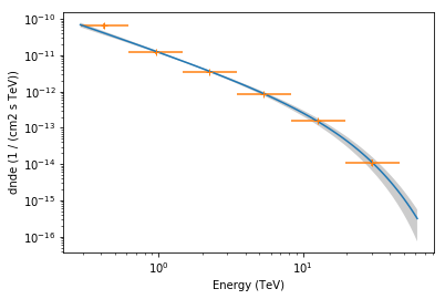
Flux points table:
e_ref e_min e_max dnde dnde_errn dnde_errp dnde_ul is_ul
TeV TeV TeV 1 / (cm2 s TeV) 1 / (cm2 s TeV) 1 / (cm2 s TeV) 1 / (cm2 s TeV)
------ ------ ------ --------------- --------------- --------------- --------------- -----
0.422 0.287 0.619 6.554e-11 1.050e-11 1.038e-11 8.637e-11 False
0.953 0.619 1.468 1.199e-11 1.292e-12 1.289e-12 1.453e-11 False
2.260 1.468 3.481 3.526e-12 2.358e-13 2.408e-13 4.018e-12 False
5.360 3.481 8.254 8.324e-13 5.496e-14 5.620e-14 9.496e-13 False
12.711 8.254 19.573 1.596e-13 1.323e-14 1.349e-14 1.870e-13 False
30.142 19.573 46.416 1.116e-14 2.189e-15 2.323e-15 1.599e-14 False
*** Gaussian component info ***
Number of components: 3
Spatial components : HGPSC 001, HGPSC 002, HGPSC 003
Component HGPSC 001:
GLON : 263.969 +/- 0.023 deg
GLAT : -3.344 +/- 0.027 deg
Size : 0.237 +/- 0.023 deg
Flux (>1 TeV) : (2.76 +/- 0.52) x 10^-12 cm^-2 s^-1 = (12.2 +/- 2.3) % Crab
Component HGPSC 002:
GLON : 263.699 +/- 0.021 deg
GLAT : -2.827 +/- 0.037 deg
Size : 0.156 +/- 0.018 deg
Flux (>1 TeV) : (1.08 +/- 0.21) x 10^-12 cm^-2 s^-1 = (4.8 +/- 0.9) % Crab
Component HGPSC 003:
GLON : 263.983 +/- 0.033 deg
GLAT : -2.997 +/- 0.046 deg
Size : 0.650 +/- 0.027 deg
Flux (>1 TeV) : (11.52 +/- 0.73) x 10^-12 cm^-2 s^-1 = (51.0 +/- 3.2) % Crab
*** Source associations info ***
Source_Name Association_Catalog Association_Name Separation
deg
-------------- ------------------- ----------------- ----------
HESS J0835-455 2FHL 2FHL J0835.3-4511 0.4737829
HESS J0835-455 3FGL 3FGL J0835.3-4510 0.48186883
HESS J0835-455 COMP G263.9-3.3 0.32130364
HESS J0835-455 PSR B0833-45 0.48390508
*** Source identification info ***
Source_Name: HESS J0835-455
Identified_Object: Vela X
Class: PWN
Evidence: Morphology
Reference: 2006A%26A...448L..43A
Distance_Reference: SNRCat
Distance: 0.2750000059604645 kpc
Distance_Min: 0.25 kpc
Distance_Max: 0.30000001192092896 kpc
In [43]:
# You can also more selectively print subsets of info:
print(source.info("map"))
*** Info from map analysis ***

RA                   :  128.887 deg = 8h35m33s
DEC                  :  -45.659 deg = -45d39m32s
GLON                 :  263.960 +/- 0.025 deg
GLAT                 :   -3.048 +/- 0.027 deg
Position Error (68%) : 0.057 deg
Position Error (95%) : 0.093 deg
ROI number           : 18
Spatial model        : 3-Gaussian
Spatial components   : HGPSC 001, HGPSC 002, HGPSC 003
TS                   : 1553.2
sqrt(TS)             : 39.4
Size                 : 0.585 +/- 0.052 (UL: nan) deg
R70                  : 0.887 deg
RSpec                : 0.500 deg
Total model excess   : 8781.6
Excess in RSpec      : 3580.1
Model Excess in RSpec : 3637.4
Background in RSpec  : 5936.9
Livetime             : 64.9 hours
Energy threshold     : 0.47 TeV
Source flux (>1 TeV) : (15.362 +/- 0.534) x 10^-12 cm^-2 s^-1 = (67.97 +/- 2.36) % Crab

Fluxes in RSpec (> 1 TeV):
Map measurement                : 5.571 x 10^-12 cm^-2 s^-1 = 24.65 % Crab
Source model                   : 5.659 x 10^-12 cm^-2 s^-1 = 25.04 % Crab
Other component model          : 0.000 x 10^-12 cm^-2 s^-1 =  0.00 % Crab
Large scale component model    : 0.000 x 10^-12 cm^-2 s^-1 =  0.00 % Crab
Total model                    : 5.659 x 10^-12 cm^-2 s^-1 = 25.04 % Crab
Containment in RSpec                :  36.8 %
Contamination in RSpec              :   0.0 %
Flux correction (RSpec -> Total)    : 271.4 %
Flux correction (Total -> RSpec)    :  36.8 %
In [44]:
# All of the data for this source is available
# via the `source.data` dictionary if you want
# to do some computations
source.data["Flux_Spec_Int_1TeV"]
Out[44]:
In [45]:
# The flux points are available as a Table
source.flux_points.table
Out[45]:
| e_ref | e_min | e_max | dnde | dnde_errn | dnde_errp | dnde_ul | is_ul |
|---|---|---|---|---|---|---|---|
| TeV | TeV | TeV | 1 / (cm2 s TeV) | 1 / (cm2 s TeV) | 1 / (cm2 s TeV) | 1 / (cm2 s TeV) | |
| float32 | float32 | float32 | float32 | float32 | float32 | float32 | bool |
| 0.4216965 | 0.28729847 | 0.6189658 | 6.5541766e-11 | 1.0499469e-11 | 1.037914e-11 | 8.636929e-11 | False |
| 0.9531619 | 0.6189658 | 1.4677993 | 1.1986031e-11 | 1.2919824e-12 | 1.2886871e-12 | 1.4526381e-11 | False |
| 2.260303 | 1.4677993 | 3.4807005 | 3.52555e-12 | 2.3576906e-13 | 2.4082174e-13 | 4.0178963e-12 | False |
| 5.360023 | 3.4807005 | 8.254042 | 8.324112e-13 | 5.495922e-14 | 5.6203943e-14 | 9.495746e-13 | False |
| 12.710618 | 8.254042 | 19.573418 | 1.5962396e-13 | 1.3232291e-14 | 1.3493189e-14 | 1.8696622e-13 | False |
| 30.141624 | 19.573418 | 46.41589 | 1.11618885e-14 | 2.1889015e-15 | 2.3228553e-15 | 1.5994852e-14 | False |
In [46]:
# The spectral model is available as a
# Gammapy spectral model object:
spectral_model = source.spectral_model()
print(spectral_model)
ExponentialCutoffPowerLaw

Parameters:

           name     value     error        unit      min max frozen
        --------- --------- --------- -------------- --- --- ------
            index 1.354e+00 7.733e-02                nan nan  False
        amplitude 6.408e-12 3.260e-13 cm-2 s-1 TeV-1 nan nan  False
        reference 1.697e+00 0.000e+00            TeV nan nan   True
          lambda_ 8.152e-02 1.154e-02          TeV-1 nan nan  False

Covariance:

           name     index   amplitude reference  lambda_
        --------- --------- --------- --------- ---------
            index 5.980e-03 0.000e+00 0.000e+00 0.000e+00
        amplitude 0.000e+00 1.063e-25 0.000e+00 0.000e+00
        reference 0.000e+00 0.000e+00 0.000e+00 0.000e+00
          lambda_ 0.000e+00 0.000e+00 0.000e+00 1.331e-04
In [47]:
# One common task is to compute integral fluxes
# The error is computed using the covariance matrix
# (off-diagonal info not given in HGPS, i.e. this is an approximation)
spectral_model.integral_error(emin=1 * u.TeV, emax=10 * u.TeV)
Out[47]:
In [48]:
# Let's plot the spectrum
source.spectral_model().plot(source.energy_range)
source.spectral_model().plot_error(source.energy_range)
source.flux_points.plot();
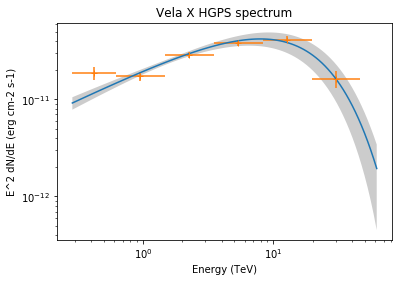
In [49]:
# Or let's make the same plot in the common
# format with y = E^2 * dnde
opts = dict(energy_power=2, flux_unit="erg-1 cm-2 s-1")
source.spectral_model().plot(source.energy_range, **opts)
source.spectral_model().plot_error(source.energy_range, **opts)
source.flux_points.plot(**opts)
plt.ylabel("E^2 dN/dE (erg cm-2 s-1)")
plt.title("Vela X HGPS spectrum");
In the next section we will see how to work with the HGPS survey maps from Gammapy, as well as work with other data from the catalog (position and morphology information).
Maps with Gammapy
Let’s use the gammapy.maps.Map.read method to load up the HGPS significance survey map.
In [50]:
path = hgps_data_path / "hgps_map_significance_0.1deg_v1.fits.gz"
survey_map = Map.read(path)
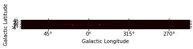
In [51]:
# Map has a quick-look plot method, but it's not
# very useful for a survey map that wide with default settings
survey_map.plot();
In [52]:
# This is a little better
fig = plt.figure(figsize=(15, 3))
_ = survey_map.plot(stretch="sqrt")
# Note that we also assign the return value (a tuple)
# from the plot method call to a variable called `_`
# This is to avoid Jupyter printing it like in the last cell,
# and generally `_` is a variable name used in Python
# for things you don't want to name or care about at all
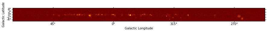
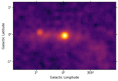
Let’s look at a cutout of the Galactic center:
In [53]:
image = survey_map.cutout(pos, width=(3.8, 2.5) * u.deg)
fig, ax, _ = image.plot(stretch="sqrt", cmap="inferno")
ax.coords[0].set_major_formatter("dd")
ax.coords[1].set_major_formatter("dd")
Side comment: If you like, you can format stuff to make it a bit more pretty. With a few lines you can get nice plots, with a few dozen publication-quality images. This is using matplotlib and astropy.visualization. Both are pretty complex, but there’s many examples available and there’s not really another good alternative anyways for astronomical sky images at the moment, so you should just go ahead and learn those.
There’s also a convenience method to look up the map value at a given sky position. Let’s repeat this for the same position we did above with Numpy and Astropy:
In [54]:
pos = SkyCoord(266.416826, -29.007797, unit="deg")
survey_map.get_by_coord(pos)
Out[54]:
array([89.49691], dtype=float32)
Vela X
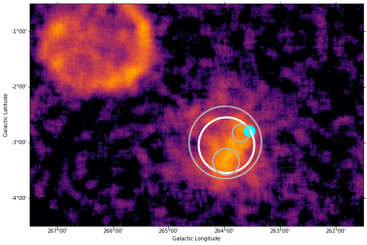
To finish up this tutorial, let’s do something a bit more advanced, than involves the survey map, the HGPS source catalog, the multi-Gauss morphology component model. Let’s show the Vela X pulsar wind nebula and the Vela Junior supernova remnant, and overplot some HGPS catalog data.
In [55]:
# The spatial model for Vela X in HGPS was three Gaussians
print(source.name)
for component in source.components:
    print(component)
HESS J0835-455
Component HGPSC 001:
GLON                 :  263.969 +/- 0.023 deg
GLAT                 :   -3.344 +/- 0.027 deg
Size                 : 0.237 +/- 0.023 deg
Flux (>1 TeV)        : (2.76 +/- 0.52) x 10^-12 cm^-2 s^-1 = (12.2 +/- 2.3) % Crab
Component HGPSC 002:
GLON                 :  263.699 +/- 0.021 deg
GLAT                 :   -2.827 +/- 0.037 deg
Size                 : 0.156 +/- 0.018 deg
Flux (>1 TeV)        : (1.08 +/- 0.21) x 10^-12 cm^-2 s^-1 = (4.8 +/- 0.9) % Crab
Component HGPSC 003:
GLON                 :  263.983 +/- 0.033 deg
GLAT                 :   -2.997 +/- 0.046 deg
Size                 : 0.650 +/- 0.027 deg
Flux (>1 TeV)        : (11.52 +/- 0.73) x 10^-12 cm^-2 s^-1 = (51.0 +/- 3.2) % Crab
In [56]:
from astropy.visualization import simple_norm
from matplotlib.patches import Circle

# Cutout and plot a nice image
pos = SkyCoord(264.5, -2.5, unit="deg", frame="galactic")
image = survey_map.cutout(pos, width=("6 deg", "4 deg"))
norm = simple_norm(image.data, stretch="sqrt", min_cut=0, max_cut=20)
fig = plt.figure(figsize=(12, 8))
fig, ax, _ = image.plot(fig=fig, norm=norm, cmap="inferno")
transform = ax.get_transform("galactic")

# Overplot the pulsar
# print(SkyCoord.from_name('Vela pulsar').galactic)
ax.scatter(263.551, -2.787, transform=transform, s=500, color="cyan")

# Overplot the circle that was used for the HGPS spectral measurement of Vela X
# It is centered on the centroid of the emission and has a radius of 0.5 deg
x = source.data["GLON"].value
y = source.data["GLAT"].value
r = source.data["RSpec"].value
c = Circle(
    (x, y), r, transform=transform, edgecolor="white", facecolor="none", lw=4
)
ax.add_patch(c)

# Overplot circles that represent the components
for c in source.components:
    x = c.data["GLON"].value
    y = c.data["GLAT"].value
    r = c.data["Size"].value
    c = Circle(
        (x, y), r, transform=transform, edgecolor="0.7", facecolor="none", lw=3
    )
    ax.add_patch(c)
We note that for HGPS there are already spatial models available:
print(source.spatial_model())
source.components[0].spatial_model
With some effort, you can use those to make HGPS model flux images.
There are two reasons we’re not showing this here: First, the spatial model code in Gammapy is work in progress, it will change soon. Secondly, doing morphology measurements on the public HGPS maps is discouraged; we note again that the maps are correlated and no detailed PSF information is published. So please be careful / conservative when extracting quantitative mesurements from the HGPS maps e.g. for a source of interest for you.
Conclusions
This concludes this tutorial how to access and work with the HGPS data from Python, using Astropy and Gammapy.
- If you have any questions about the HGPS data, please use the contact given at https://www.mpi-hd.mpg.de/hfm/HESS/hgps/ .
- If you have any questions or issues about Astropy or Gammapy, please use the Gammapy mailing list (see https://gammapy.org/contact.html).
Please read the Appendix A of the paper to learn about the caveats to using the HGPS data. Especially note that the HGPS survey maps are correlated and thus no detailed source morphology analysis is possible, and also note the caveats concerning spectral models and spectral flux points.
Exercises
- Re-run this notebook, but change the HGPS source that was used for examples. If you have any questions about the data, try to access and print or plot it. Just to give a few ideas: How many identified pulsar wind nebulae are in HGPS? Which are the 5 brightest HGPS sources in the 1-10 TeV energy band? Which is the second-highest significance source in the HPGS image after the Galactic center?
- Try to reproduce some of the figures in the HGPS paper. Don’t try to reproduce them exactly, but just try to write ~ 10 lines of code to access the relevant HGPS data and make a quick plot that shows the same or similar information.
- Fit a spectral model to the spectral points of Vela X and compare with the HGPS model fit. (they should be similar, but not identical, in HGPS a likelihood fit to counts data was done). For this task, the spectrum_models and sed_fitting_gammacat_fermi tutorials will be useful.
In [57]: