This is a fixed-text formatted version of a Jupyter notebook

• Try online

• You may download all the notebooks as a tar file.

• Source files: spectrum_simulation.ipynb | spectrum_simulation.py

1D spectrum simulation

Prerequisites

• Knowledge of spectral extraction and datasets used in gammapy, see for instance the spectral analysis tutorial

Context

To simulate a specific observation, it is not always necessary to simulate the full photon list. For many uses cases, simulating directly a reduced binned dataset is enough: the IRFs reduced in the correct geometry are combined with a source model to predict an actual number of counts per bin. The latter is then used to simulate a reduced dataset using Poisson probability distribution.

This can be done to check the feasibility of a measurement, to test whether fitted parameters really provide a good fit to the data etc.

Here we will see how to perform a 1D spectral simulation of a CTA observation, in particular, we will generate OFF observations following the template background stored in the CTA IRFs.

Objective: simulate a number of spectral ON-OFF observations of a source with a power-law spectral model with CTA using the CTA 1DC response, fit them with the assumed spectral model and check that the distribution of fitted parameters is consistent with the input values.

Proposed approach

We will use the following classes:

• gammapy.datasets.SpectrumDatasetOnOff

• gammapy.datasets.SpectrumDataset

• gammapy.irf.load_cta_irfs

• gammapy.modeling.models.PowerLawSpectralModel

Setup

%matplotlib inline
import matplotlib.pyplot as plt

import numpy as np
import astropy.units as u
from astropy.coordinates import SkyCoord, Angle
from regions import CircleSkyRegion
from gammapy.datasets import SpectrumDatasetOnOff, SpectrumDataset, Datasets
from gammapy.makers import SpectrumDatasetMaker
from gammapy.modeling import Fit
from gammapy.modeling.models import (
    PowerLawSpectralModel,
    SkyModel,
)
from gammapy.irf import load_cta_irfs
from gammapy.data import Observation, observatory_locations
from gammapy.maps import MapAxis, RegionGeom

Simulation of a single spectrum

To do a simulation, we need to define the observational parameters like the livetime, the offset, the assumed integration radius, the energy range to perform the simulation for and the choice of spectral model. We then use an in-memory observation which is convolved with the IRFs to get the predicted number of counts. This is Poission fluctuated using the fake() to get the simulated counts for each observation.

# Define simulation parameters parameters
livetime = 1 * u.h

pointing = SkyCoord(0, 0, unit="deg", frame="galactic")
offset = 0.5 * u.deg

# Reconstructed and true energy axis
energy_axis = MapAxis.from_edges(
    np.logspace(-0.5, 1.0, 10), unit="TeV", name="energy", interp="log"
)
energy_axis_true = MapAxis.from_edges(
    np.logspace(-1.2, 2.0, 31), unit="TeV", name="energy_true", interp="log"
)

on_region_radius = Angle("0.11 deg")

center = pointing.directional_offset_by(
    position_angle=0 * u.deg, separation=offset
)
on_region = CircleSkyRegion(center=center, radius=on_region_radius)

# Define spectral model - a simple Power Law in this case
model_simu = PowerLawSpectralModel(
    index=3.0,
    amplitude=2.5e-12 * u.Unit("cm-2 s-1 TeV-1"),
    reference=1 * u.TeV,
)
print(model_simu)
# we set the sky model used in the dataset
model = SkyModel(spectral_model=model_simu, name="source")

PowerLawSpectralModel

  type      name     value         unit        error   min max frozen is_norm link
-------- --------- ---------- -------------- --------- --- --- ------ ------- ----
spectral     index 3.0000e+00                0.000e+00 nan nan  False   False
spectral amplitude 2.5000e-12 cm-2 s-1 TeV-1 0.000e+00 nan nan  False    True
spectral reference 1.0000e+00            TeV 0.000e+00 nan nan   True   False

# Load the IRFs
# In this simulation, we use the CTA-1DC irfs shipped with gammapy.
irfs = load_cta_irfs(
    "$GAMMAPY_DATA/cta-1dc/caldb/data/cta/1dc/bcf/South_z20_50h/irf_file.fits"
)

Invalid unit found in background table! Assuming (s-1 MeV-1 sr-1)

location = observatory_locations["cta_south"]
obs = Observation.create(
    pointing=pointing,
    livetime=livetime,
    irfs=irfs,
    location=location,
)
print(obs)

Observation

        obs id            : 0
        tstart            : 51544.00
        tstop             : 51544.04
        duration          : 3600.00 s
        pointing (icrs)   : 266.4 deg, -28.9 deg

        deadtime fraction : 0.0%

# Make the SpectrumDataset
geom = RegionGeom.create(region=on_region, axes=[energy_axis])

dataset_empty = SpectrumDataset.create(
    geom=geom, energy_axis_true=energy_axis_true, name="obs-0"
)
maker = SpectrumDatasetMaker(selection=["exposure", "edisp", "background"])

dataset = maker.run(dataset_empty, obs)

# Set the model on the dataset, and fake
dataset.models = model
dataset.fake(random_state=42)
print(dataset)

SpectrumDataset
---------------

  Name                            : obs-0

  Total counts                    : 298
  Total background counts         : 22.29
  Total excess counts             : 275.71

  Predicted counts                : 303.66
  Predicted background counts     : 22.29
  Predicted excess counts         : 281.37

  Exposure min                    : 2.53e+08 m2 s
  Exposure max                    : 1.77e+10 m2 s

  Number of total bins            : 9
  Number of fit bins              : 9

  Fit statistic type              : cash
  Fit statistic value (-2 log(L)) : -1811.58

  Number of models                : 1
  Number of parameters            : 3
  Number of free parameters       : 2

  Component 0: SkyModel

    Name                      : source
    Datasets names            : None
    Spectral model type       : PowerLawSpectralModel
    Spatial  model type       :
    Temporal model type       :
    Parameters:
      index                         :      3.000   +/-    0.00
      amplitude                     :   2.50e-12   +/- 0.0e+00 1 / (cm2 s TeV)
      reference             (frozen):      1.000       TeV

You can see that background counts are now simulated

On-Off analysis

To do an on off spectral analysis, which is the usual science case, the standard would be to use SpectrumDatasetOnOff, which uses the acceptance to fake off-counts

dataset_on_off = SpectrumDatasetOnOff.from_spectrum_dataset(
    dataset=dataset, acceptance=1, acceptance_off=5
)
dataset_on_off.fake(npred_background=dataset.npred_background())
print(dataset_on_off)

SpectrumDatasetOnOff
--------------------

  Name                            : HEEdFEpA

  Total counts                    : 314
  Total background counts         : 22.40
  Total excess counts             : 291.60

  Predicted counts                : 303.82
  Predicted background counts     : 22.45
  Predicted excess counts         : 281.37

  Exposure min                    : 2.53e+08 m2 s
  Exposure max                    : 1.77e+10 m2 s

  Number of total bins            : 9
  Number of fit bins              : 9

  Fit statistic type              : wstat
  Fit statistic value (-2 log(L)) : 10.32

  Number of models                : 1
  Number of parameters            : 3
  Number of free parameters       : 2

  Component 0: SkyModel

    Name                      : source
    Datasets names            : None
    Spectral model type       : PowerLawSpectralModel
    Spatial  model type       :
    Temporal model type       :
    Parameters:
      index                         :      3.000   +/-    0.00
      amplitude                     :   2.50e-12   +/- 0.0e+00 1 / (cm2 s TeV)
      reference             (frozen):      1.000       TeV

    Total counts_off                : 112
  Acceptance                      : 9
  Acceptance off                  : 45

You can see that off counts are now simulated as well. We now simulate several spectra using the same set of observation conditions.

%%time

n_obs = 100
datasets = Datasets()

for idx in range(n_obs):
    dataset_on_off.fake(
        random_state=idx, npred_background=dataset.npred_background()
    )
    dataset_fake = dataset_on_off.copy(name=f"obs-{idx}")
    dataset_fake.meta_table["OBS_ID"] = [idx]
    datasets.append(dataset_fake)

CPU times: user 2.36 s, sys: 43.2 ms, total: 2.41 s
Wall time: 2.67 s

table = datasets.info_table()
table

Table length=100

name	counts	excess	sqrt_ts	background	npred	npred_background	npred_signal	exposure_min	exposure_max	livetime	ontime	counts_rate	background_rate	excess_rate	n_bins	n_fit_bins	stat_type	stat_sum	counts_off	acceptance	acceptance_off	alpha
								m2 s	m2 s	s	s	1 / s	1 / s	1 / s
str6	int64	float64	float64	float64	float64	float64	float64	float64	float64	float64	float64	float64	float64	float64	int64	int64	str5	float64	int64	float64	float64	float64
obs-0	317	298.6000061035156	27.08240180813126	18.399999618530273	68.16666751313541	68.16666751313541	nan	252718176.0	17719697408.0	3600.000000000002	3600.000000000002	0.08805555555555551	0.0051111110051472956	0.08294444613986542	9	9	wstat	738.7245834271496	92	9.0	45.0	0.20000000298023224
obs-1	275	253.0	23.76785365487285	22.0	64.16666666666669	64.16666666666669	nan	252718170.97287694	17719697919.59929	3600.000000000002	3600.000000000002	0.07638888888888885	0.006111111111111108	0.07027777777777774	9	9	wstat	575.779512784738	110	9.0	45.0	0.2
obs-2	293	272.4	25.17110555404655	20.6	66.0	66.0	nan	252718170.97287694	17719697919.59929	3600.000000000002	3600.000000000002	0.08138888888888884	0.00572222222222222	0.07566666666666662	9	9	wstat	645.4993824075303	103	9.0	45.0	0.2
obs-3	280	257.6	23.982951737405354	22.4	65.33333333333334	65.33333333333334	nan	252718170.97287694	17719697919.59929	3600.000000000002	3600.000000000002	0.07777777777777774	0.006222222222222218	0.07155555555555553	9	9	wstat	585.9241546985872	112	9.0	45.00000000000001	0.19999999999999998
obs-4	337	316.4	27.682709945184747	20.6	73.33333333333334	73.33333333333334	nan	252718170.97287694	17719697919.59929	3600.000000000002	3600.000000000002	0.09361111111111106	0.00572222222222222	0.08788888888888884	9	9	wstat	787.314723949448	103	9.0	45.0	0.2
obs-5	283	258.6	23.727154782347895	24.400000000000002	67.50000000000001	67.50000000000001	nan	252718170.97287694	17719697919.59929	3600.000000000002	3600.000000000002	0.07861111111111108	0.006777777777777775	0.0718333333333333	9	9	wstat	574.8525737727499	122	9.0	45.0	0.2
obs-6	330	307.6	26.889184475727866	22.400000000000006	73.66666666666667	73.66666666666667	nan	252718170.97287694	17719697919.59929	3600.000000000002	3600.000000000002	0.09166666666666662	0.006222222222222221	0.0854444444444444	9	9	wstat	734.2414755285937	112	9.0	44.99999999999999	0.20000000000000004
obs-7	283	257.2	23.43087974795853	25.8	68.66666666666667	68.66666666666667	nan	252718170.97287694	17719697919.59929	3600.000000000002	3600.000000000002	0.07861111111111108	0.007166666666666663	0.07144444444444441	9	9	wstat	552.3698779448044	129	9.0	45.0	0.2
obs-8	308	284.6	25.42049273328331	23.400000000000002	70.83333333333334	70.83333333333334	nan	252718170.97287694	17719697919.59929	3600.000000000002	3600.000000000002	0.08555555555555551	0.006499999999999997	0.07905555555555552	9	9	wstat	652.2621572567633	117	9.0	45.0	0.2
obs-9	299	278.6	25.57085071486863	20.4	66.83333333333334	66.83333333333334	nan	252718170.97287694	17719697919.59929	3600.000000000002	3600.000000000002	0.08305555555555551	0.005666666666666664	0.07738888888888885	9	9	wstat	666.9062670260786	102	9.0	45.00000000000001	0.19999999999999998
obs-10	310	294.8	27.488972161356774	15.2	64.33333333333334	64.33333333333334	nan	252718170.97287694	17719697919.59929	3600.000000000002	3600.000000000002	0.08611111111111107	0.00422222222222222	0.08188888888888884	9	9	wstat	768.5404492529331	76	9.0	45.00000000000001	0.19999999999999998
obs-11	285	261.0	23.933833745454685	24.000000000000004	67.50000000000001	67.50000000000001	nan	252718170.97287694	17719697919.59929	3600.000000000002	3600.000000000002	0.07916666666666662	0.0066666666666666645	0.07249999999999997	9	9	wstat	583.448753292733	120	9.0	44.99999999999999	0.20000000000000004
obs-12	299	278.0	25.4325263895117	21.000000000000004	67.33333333333336	67.33333333333336	nan	252718170.97287694	17719697919.59929	3600.000000000002	3600.000000000002	0.08305555555555551	0.005833333333333331	0.07722222222222218	9	9	wstat	655.2768246480357	105	9.0	44.99999999999999	0.20000000000000004
obs-13	309	287.4	25.877406235012618	21.6	69.50000000000001	69.50000000000001	nan	252718170.97287694	17719697919.59929	3600.000000000002	3600.000000000002	0.08583333333333329	0.0059999999999999975	0.07983333333333328	9	9	wstat	672.355748274336	108	9.0	45.0	0.2
...	...	...	...	...	...	...	...	...	...	...	...	...	...	...	...	...	...	...	...	...	...	...
obs-85	297	274.6	24.998935845735573	22.4	68.16666666666667	68.16666666666667	nan	252718170.97287694	17719697919.59929	3600.000000000002	3600.000000000002	0.08249999999999996	0.006222222222222218	0.07627777777777775	9	9	wstat	631.6298361198053	112	9.0	45.00000000000001	0.19999999999999998
obs-86	286	268.2	25.42340896951546	17.800000000000004	62.50000000000001	62.50000000000001	nan	252718170.97287694	17719697919.59929	3600.000000000002	3600.000000000002	0.0794444444444444	0.004944444444444443	0.07449999999999996	9	9	wstat	655.2082535886425	89	9.0	44.99999999999999	0.20000000000000004
obs-87	333	313.2	27.646851451147217	19.8	72.00000000000001	72.00000000000001	nan	252718170.97287694	17719697919.59929	3600.000000000002	3600.000000000002	0.09249999999999996	0.005499999999999997	0.08699999999999995	9	9	wstat	770.1313412321031	99	9.0	45.0	0.2
obs-88	315	296.8	27.0172059251097	18.200000000000003	67.66666666666669	67.66666666666669	nan	252718170.97287694	17719697919.59929	3600.000000000002	3600.000000000002	0.08749999999999995	0.005055555555555554	0.0824444444444444	9	9	wstat	734.6476098262428	91	9.0	44.99999999999999	0.20000000000000004
obs-89	287	265.0	24.49456558680515	22.000000000000004	66.16666666666667	66.16666666666667	nan	252718170.97287694	17719697919.59929	3600.000000000002	3600.000000000002	0.07972222222222218	0.006111111111111109	0.07361111111111107	9	9	wstat	611.2334063685089	110	9.0	44.99999999999999	0.20000000000000004
obs-90	286	267.0	25.131221887043438	19.000000000000004	63.50000000000001	63.50000000000001	nan	252718170.97287694	17719697919.59929	3600.000000000002	3600.000000000002	0.0794444444444444	0.005277777777777776	0.07416666666666663	9	9	wstat	635.8304116110406	95	9.0	44.99999999999999	0.20000000000000004
obs-91	285	259.8	23.67754591931069	25.200000000000003	68.50000000000001	68.50000000000001	nan	252718170.97287694	17719697919.59929	3600.000000000002	3600.000000000002	0.07916666666666662	0.0069999999999999975	0.07216666666666663	9	9	wstat	573.3564742963381	126	9.0	45.0	0.2
obs-92	313	289.4	25.664935420194176	23.6	71.83333333333336	71.83333333333336	nan	252718170.97287694	17719697919.59929	3600.000000000002	3600.000000000002	0.0869444444444444	0.006555555555555552	0.08038888888888884	9	9	wstat	669.4496142825196	118	9.0	45.0	0.2
obs-93	302	283.2	26.123867522605497	18.8	66.00000000000001	66.00000000000001	nan	252718170.97287694	17719697919.59929	3600.000000000002	3600.000000000002	0.08388888888888885	0.00522222222222222	0.07866666666666662	9	9	wstat	700.5066738339824	94	9.0	45.0	0.2
obs-94	322	300.2	26.574029757473202	21.8	71.83333333333334	71.83333333333334	nan	252718170.97287694	17719697919.59929	3600.000000000002	3600.000000000002	0.0894444444444444	0.006055555555555553	0.08338888888888885	9	9	wstat	715.2570498037147	109	9.0	45.0	0.2
obs-95	305	280.6	25.030731260493152	24.400000000000006	71.16666666666667	71.16666666666667	nan	252718170.97287694	17719697919.59929	3600.000000000002	3600.000000000002	0.08472222222222218	0.006777777777777776	0.07794444444444441	9	9	wstat	643.2846879404793	122	9.0	44.99999999999999	0.20000000000000004
obs-96	301	277.4	24.969845969421428	23.6	69.83333333333334	69.83333333333334	nan	252718170.97287694	17719697919.59929	3600.000000000002	3600.000000000002	0.08361111111111107	0.006555555555555552	0.07705555555555552	9	9	wstat	626.7396842428624	118	9.0	45.0	0.2
obs-97	290	271.2	25.417982194454826	18.8	64.00000000000001	64.00000000000001	nan	252718170.97287694	17719697919.59929	3600.000000000002	3600.000000000002	0.08055555555555552	0.00522222222222222	0.0753333333333333	9	9	wstat	650.9762484493856	94	9.0	45.0	0.2
obs-98	301	280.6	25.687832964675007	20.400000000000002	67.16666666666667	67.16666666666667	nan	252718170.97287694	17719697919.59929	3600.000000000002	3600.000000000002	0.08361111111111107	0.0056666666666666645	0.07794444444444441	9	9	wstat	664.5620099404952	102	9.0	45.0	0.2
obs-99	323	302.2	26.85707842376871	20.8	71.16666666666669	71.16666666666669	nan	252718170.97287694	17719697919.59929	3600.000000000002	3600.000000000002	0.08972222222222218	0.005777777777777775	0.0839444444444444	9	9	wstat	733.1576598768017	104	9.0	45.0	0.2

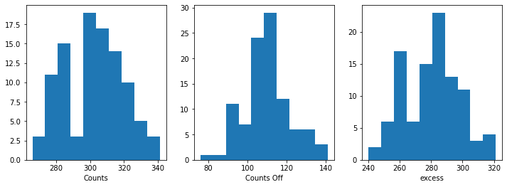
Before moving on to the fit let’s have a look at the simulated observations.

fix, axes = plt.subplots(1, 3, figsize=(12, 4))
axes[0].hist(table["counts"])
axes[0].set_xlabel("Counts")
axes[1].hist(table["counts_off"])
axes[1].set_xlabel("Counts Off")
axes[2].hist(table["excess"])
axes[2].set_xlabel("excess");

Now, we fit each simulated spectrum individually

%%time
results = []

fit = Fit()

for dataset in datasets:
    dataset.models = model.copy()
    result = fit.optimize(dataset)
    results.append(
        {
            "index": result.parameters["index"].value,
            "amplitude": result.parameters["amplitude"].value,
        }
    )

CPU times: user 40.7 s, sys: 247 ms, total: 40.9 s
Wall time: 45.1 s

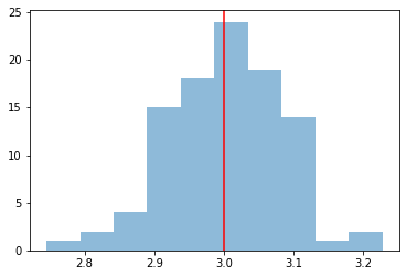
We take a look at the distribution of the fitted indices. This matches very well with the spectrum that we initially injected.

index = np.array([_["index"] for _ in results])
plt.hist(index, bins=10, alpha=0.5)
plt.axvline(x=model_simu.parameters["index"].value, color="red")
print(f"index: {index.mean()} += {index.std()}")

index: 3.003692555041602 += 0.08081469526978655

Exercises

• Change the observation time to something longer or shorter. Does the observation and spectrum results change as you expected?

• Change the spectral model, e.g. add a cutoff at 5 TeV, or put a steep-spectrum source with spectral index of 4.0

• Simulate spectra with the spectral model we just defined. How much observation duration do you need to get back the injected parameters?