This is a fixed-text formatted version of a Jupyter notebook

• Try online

• You may download all the notebooks as a tar file.

• Source files: light_curve_simulation.ipynb | light_curve_simulation.py

Simulating and fitting a time varying source

Prerequisites

• To understand how a single binned simulation works, please refer to spectrum_simulation simulate_3d for 1D and 3D simulations respectively.

• For details of light curve extraction using gammapy, refer to the two tutorials light_curve and light_curve_flare

Context

Frequently, studies of variable sources (eg: decaying GRB light curves, AGN flares, etc) require time variable simulations. For most use cases, generating an event list is an overkill, and it suffices to use binned simulations using a temporal model.

Objective: Simulate and fit a time decaying light curve of a source with CTA using the CTA 1DC response

Proposed approach

We will simulate 10 spectral datasets within given time intervals (Good Time Intervals) following a given spectral (a power law) and temporal profile (an exponential decay, with a decay time of 6 hr ). These are then analysed using the light curve estimator to obtain flux points.

Modelling and fitting of lightcurves can be done either - directly on the output of the LighCurveEstimator (at the DL5 level) - fit the simulated datasets (at the DL4 level)

In summary, necessary steps are:

• Choose observation parameters including a list of gammapy.data.GTI

• Define temporal and spectral models from :ref:model-gallery as per science case

• Perform the simulation (in 1D or 3D)

• Extract the light curve from the reduced dataset as shown in light curve notebook

• Optionally, we show here how to fit the simulated datasets using a source model

Setup

As usual, we’ll start with some general imports…

Setup

%matplotlib inline
import matplotlib.pyplot as plt
import numpy as np
import astropy.units as u
from astropy.coordinates import SkyCoord
from astropy.time import Time

import logging

log = logging.getLogger(__name__)

And some gammapy specific imports

from gammapy.data import Observation
from gammapy.irf import load_cta_irfs
from gammapy.datasets import SpectrumDataset, Datasets, FluxPointsDataset
from gammapy.modeling.models import (
    PowerLawSpectralModel,
    ExpDecayTemporalModel,
    SkyModel,
)
from gammapy.maps import MapAxis, RegionGeom, TimeMapAxis
from gammapy.estimators import LightCurveEstimator
from gammapy.makers import SpectrumDatasetMaker
from gammapy.modeling import Fit
from gammapy.data import observatory_locations

We first define our preferred time format:

TimeMapAxis.time_format = "iso"

Simulating a light curve

We will simulate 10 spectra between 300 GeV and 10 TeV using an PowerLawSpectralModel and a ExpDecayTemporalModel. The important thing to note here is how to attach a different GTI to each dataset. Since we use spectrum datasets here, we will use a RegionGeom.

# Loading IRFs
irfs = load_cta_irfs(
    "$GAMMAPY_DATA/cta-1dc/caldb/data/cta/1dc/bcf/South_z20_50h/irf_file.fits"
)

Invalid unit found in background table! Assuming (s-1 MeV-1 sr-1)

# Reconstructed and true energy axis
energy_axis = MapAxis.from_edges(
    np.logspace(-0.5, 1.0, 10), unit="TeV", name="energy", interp="log"
)
energy_axis_true = MapAxis.from_edges(
    np.logspace(-1.2, 2.0, 31), unit="TeV", name="energy_true", interp="log"
)

geom = RegionGeom.create("galactic;circle(0, 0, 0.11)", axes=[energy_axis])

# Pointing position
pointing = SkyCoord(0.5, 0.5, unit="deg", frame="galactic")

Note that observations are usually conducted in Wobble mode, in which the source is not in the center of the camera. This allows to have a symmetrical sky position from which background can be estimated.

# Define the source model: A combination of spectral and temporal model

gti_t0 = Time("2020-03-01")
spectral_model = PowerLawSpectralModel(
    index=3, amplitude="1e-11 cm-2 s-1 TeV-1", reference="1 TeV"
)
temporal_model = ExpDecayTemporalModel(t0="6 h", t_ref=gti_t0.mjd * u.d)

model_simu = SkyModel(
    spectral_model=spectral_model,
    temporal_model=temporal_model,
    name="model-simu",
)

/Users/terrier/Code/anaconda3/envs/gammapy-dev/lib/python3.8/site-packages/astropy/units/quantity.py:613: RuntimeWarning: overflow encountered in exp
  result = super().__array_ufunc__(function, method, *arrays, **kwargs)
/Users/terrier/Code/anaconda3/envs/gammapy-dev/lib/python3.8/site-packages/astropy/units/quantity.py:613: RuntimeWarning: invalid value encountered in subtract
  result = super().__array_ufunc__(function, method, *arrays, **kwargs)

# Look at the model
model_simu.parameters.to_table()

Table length=5

type	name	value	unit	error	min	max	frozen	is_norm	link
str8	str9	float64	str14	int64	float64	float64	bool	bool	str1
spectral	index	3.0000e+00		0.000e+00	nan	nan	False	False
spectral	amplitude	1.0000e-11	cm-2 s-1 TeV-1	0.000e+00	nan	nan	False	True
spectral	reference	1.0000e+00	TeV	0.000e+00	nan	nan	True	False
temporal	t0	6.0000e+00	h	0.000e+00	nan	nan	False	False
temporal	t_ref	5.8909e+04	d	0.000e+00	nan	nan	True	False

Now, define the start and observation livetime wrt to the reference time, gti_t0

n_obs = 10

tstart = gti_t0 + [1, 2, 3, 5, 8, 10, 20, 22, 23, 24] * u.h
lvtm = [55, 25, 26, 40, 40, 50, 40, 52, 43, 47] * u.min

Now perform the simulations

datasets = Datasets()

empty = SpectrumDataset.create(
    geom=geom, energy_axis_true=energy_axis_true, name="empty"
)

maker = SpectrumDatasetMaker(selection=["exposure", "background", "edisp"])


for idx in range(n_obs):
    obs = Observation.create(
        pointing=pointing,
        livetime=lvtm[idx],
        tstart=tstart[idx],
        irfs=irfs,
        reference_time=gti_t0,
        obs_id=idx,
        location=observatory_locations["cta_south"],
    )
    empty_i = empty.copy(name=f"dataset-{idx}")
    dataset = maker.run(empty_i, obs)
    dataset.models = model_simu
    dataset.fake()
    datasets.append(dataset)

The reduced datasets have been successfully simulated. Let’s take a quick look into our datasets.

datasets.info_table()

Table length=10

name	counts	excess	sqrt_ts	background	npred	npred_background	npred_signal	exposure_min	exposure_max	livetime	ontime	counts_rate	background_rate	excess_rate	n_bins	n_fit_bins	stat_type	stat_sum
								m2 s	m2 s	s	s	1 / s	1 / s	1 / s
str9	int64	float64	float64	float64	float64	float64	float64	float64	float64	float64	float64	float64	float64	float64	int64	int64	str4	float64
dataset-0	829	808.6812133789062	67.31731458104936	20.318769454956055	20.318769469857216	20.318769454956055	nan	216137904.0	16025275392.0	3299.9999999999973	3300.0	0.25121212121212144	0.006157202865138204	0.24505491314512332	9	9	cash	nan
dataset-1	330	320.7641959176923	41.4564216021322	9.235804082307682	332.1496126848936	9.235804082307682	322.91380860258596	98244500.93556362	7284216297.312286	1500.0000000000036	1500.0000000000036	0.21999999999999947	0.00615720272153844	0.213842797278461	9	9	cash	-2053.5263391934623
dataset-2	320	310.3947637544	40.28720068338956	9.60523624559999	293.48960245451894	9.60523624559999	283.884366208919	102174280.97298616	7575584949.204778	1560.0000000000036	1560.0000000000036	0.20512820512820465	0.006157202721538441	0.1989710024066662	9	9	cash	-1995.2213487608487
dataset-3	320	305.22271346830775	36.847002227816574	14.777286531692258	321.7838592189118	14.777286531692258	307.00657268721955	157191201.49690142	11654746075.69963	2400.0	2400.0	0.13333333333333333	0.006157202721538441	0.1271761306117949	9	9	cash	-1950.1409750273895
dataset-4	213	198.22271346830775	27.20676640833841	14.777286531692258	200.9861855997861	14.777286531692258	186.2088990680938	157191201.49690142	11654746075.69963	2400.0	2400.0	0.08875	0.006157202721538441	0.08259279727846155	9	9	cash	-1137.4784918388684
dataset-5	190	171.52839183538467	23.294701482664998	18.471608164615322	182.99944247949256	18.471608164615322	164.5278343148772	196489001.87112677	14568432594.624538	3000.0	3000.0	0.06333333333333334	0.006157202721538441	0.05717613061179489	9	9	cash	-1016.7012114582753
dataset-6	38	23.22271346830774	5.033505913945236	14.777286531692258	39.977920628250665	14.777286531692258	25.20063409655841	157191201.49690142	11654746075.69963	2400.0	2400.0	0.015833333333333335	0.006157202721538441	0.009676130611794892	9	9	cash	-64.33017421792906
dataset-7	51	31.789527508800063	6.00089086025525	19.210472491199937	42.30482855222412	19.210472491199937	23.094356061024193	204348561.94597185	15151169898.40952	3120.0	3120.0	0.016346153846153847	0.0061572027215384415	0.010188951124615405	9	9	cash	-137.61176114657297
dataset-8	31	15.114416978430823	3.350049342927064	15.885583021569177	32.249900287793274	15.885583021569177	16.36431726622409	168980541.609169	12528852031.377102	2580.0	2580.0	0.012015503875968992	0.006157202721538441	0.0058583011544305515	9	9	cash	-53.98618916042473
dataset-9	39	21.6366883252616	4.45470472668954	17.3633116747384	32.421834962248106	17.3633116747384	15.05852328750971	184699661.75885916	13694326638.947065	2820.0	2820.0	0.013829787234042552	0.006157202721538441	0.007672584512504113	9	9	cash	-84.26051818568244

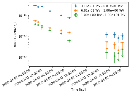
Extract the lightcurve

This section uses standard light curve estimation tools for a 1D extraction. Only a spectral model needs to be defined in this case. Since the estimator returns the integrated flux separately for each time bin, the temporal model need not be accounted for at this stage. We extract the lightcurve in 3 energy binsç

# Define the model:
spectral_model = PowerLawSpectralModel(
    index=3, amplitude="1e-11 cm-2 s-1 TeV-1", reference="1 TeV"
)
model_fit = SkyModel(spectral_model=spectral_model, name="model-fit")

# Attach model to all datasets
datasets.models = model_fit

%%time
lc_maker_1d = LightCurveEstimator(
    energy_edges=[0.3, 0.6, 1.0, 10] * u.TeV,
    source="model-fit",
    selection_optional=["ul"],
)
lc_1d = lc_maker_1d.run(datasets)

CPU times: user 26.1 s, sys: 238 ms, total: 26.3 s
Wall time: 30.1 s

ax = lc_1d.plot(marker="o", axis_name="time", sed_type="flux")

Fitting temporal models

We have the reconstructed lightcurve at this point. Now we want to fit a profile to the obtained light curves, using a joint fitting across the different datasets, while simultaneously minimising across the temporal model parameters as well. The temporal models can be applied

• directly on the obtained lightcurve

• on the simulated datasets

Fitting the obtained light curve

The fitting will proceed through a joint fit of the flux points. First, we need to obtain a set of FluxPointDatasets, one for each time bin

## Create the datasets by iterating over the returned lightcurve
datasets = Datasets()

for idx, fp in enumerate(lc_1d.iter_by_axis(axis_name="time")):
    dataset = FluxPointsDataset(data=fp, name=f"time-bin-{idx}")
    datasets.append(dataset)

We will fit the amplitude, spectral index and the decay time scale. Note that t_ref should be fixed by default for the ExpDecayTemporalModel.

# Define the model:
spectral_model1 = PowerLawSpectralModel(
    index=2.0, amplitude="1e-12 cm-2 s-1 TeV-1", reference="1 TeV"
)
temporal_model1 = ExpDecayTemporalModel(t0="10 h", t_ref=gti_t0.mjd * u.d)

model = SkyModel(
    spectral_model=spectral_model1,
    temporal_model=temporal_model1,
    name="model-test",
)

/Users/terrier/Code/anaconda3/envs/gammapy-dev/lib/python3.8/site-packages/astropy/units/quantity.py:613: RuntimeWarning: overflow encountered in exp
  result = super().__array_ufunc__(function, method, *arrays, **kwargs)
/Users/terrier/Code/anaconda3/envs/gammapy-dev/lib/python3.8/site-packages/astropy/units/quantity.py:613: RuntimeWarning: invalid value encountered in subtract
  result = super().__array_ufunc__(function, method, *arrays, **kwargs)

datasets.models = model

%%time
# Do a joint fit
fit = Fit()
result = fit.run(datasets=datasets)

CPU times: user 25.4 s, sys: 239 ms, total: 25.6 s
Wall time: 33.5 s

/Users/terrier/Code/anaconda3/envs/gammapy-dev/lib/python3.8/site-packages/astropy/units/quantity.py:613: RuntimeWarning: overflow encountered in exp
  result = super().__array_ufunc__(function, method, *arrays, **kwargs)
/Users/terrier/Code/anaconda3/envs/gammapy-dev/lib/python3.8/site-packages/astropy/units/quantity.py:613: RuntimeWarning: invalid value encountered in subtract
  result = super().__array_ufunc__(function, method, *arrays, **kwargs)

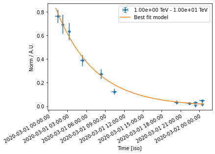
Now let’s plot model and data. We plot only the normalisation of the temporal model in relative units for one particular energy range

lc_1TeV_10TeV = lc_1d.slice_by_idx({"energy": slice(2, 3)})
ax = lc_1TeV_10TeV.plot(sed_type="norm", axis_name="time")

time_range = lc_1TeV_10TeV.geom.axes["time"].time_bounds
temporal_model1.plot(ax=ax, time_range=time_range, label="Best fit model")

ax.set_yscale("linear")
plt.legend()

<matplotlib.legend.Legend at 0x143f0b700>

Fit the datasets

Here, we apply the models directly to the simulated datasets.

For modelling and fitting more complex flares, you should attach the relevant model to each group of datasets. The parameters of a model in a given group of dataset will be tied. For more details on joint fitting in gammapy, see here.

# Define the model:
spectral_model2 = PowerLawSpectralModel(
    index=2.0, amplitude="1e-12 cm-2 s-1 TeV-1", reference="1 TeV"
)
temporal_model2 = ExpDecayTemporalModel(t0="10 h", t_ref=gti_t0.mjd * u.d)

model2 = SkyModel(
    spectral_model=spectral_model2,
    temporal_model=temporal_model2,
    name="model-test2",
)

/Users/terrier/Code/anaconda3/envs/gammapy-dev/lib/python3.8/site-packages/astropy/units/quantity.py:613: RuntimeWarning: overflow encountered in exp
  result = super().__array_ufunc__(function, method, *arrays, **kwargs)
/Users/terrier/Code/anaconda3/envs/gammapy-dev/lib/python3.8/site-packages/astropy/units/quantity.py:613: RuntimeWarning: invalid value encountered in subtract
  result = super().__array_ufunc__(function, method, *arrays, **kwargs)

model2.parameters.to_table()

Table length=5

type	name	value	unit	error	min	max	frozen	is_norm	link
str8	str9	float64	str14	int64	float64	float64	bool	bool	str1
spectral	index	2.0000e+00		0.000e+00	nan	nan	False	False
spectral	amplitude	1.0000e-12	cm-2 s-1 TeV-1	0.000e+00	nan	nan	False	True
spectral	reference	1.0000e+00	TeV	0.000e+00	nan	nan	True	False
temporal	t0	1.0000e+01	h	0.000e+00	nan	nan	False	False
temporal	t_ref	5.8909e+04	d	0.000e+00	nan	nan	True	False

datasets.models = model2

%%time
# Do a joint fit
fit = Fit()
result = fit.run(datasets=datasets)

CPU times: user 21.5 s, sys: 82.6 ms, total: 21.5 s
Wall time: 23.2 s

/Users/terrier/Code/anaconda3/envs/gammapy-dev/lib/python3.8/site-packages/astropy/units/quantity.py:613: RuntimeWarning: overflow encountered in exp
  result = super().__array_ufunc__(function, method, *arrays, **kwargs)
/Users/terrier/Code/anaconda3/envs/gammapy-dev/lib/python3.8/site-packages/astropy/units/quantity.py:613: RuntimeWarning: invalid value encountered in subtract
  result = super().__array_ufunc__(function, method, *arrays, **kwargs)

result.parameters.to_table()

Table length=5

type	name	value	unit	error	min	max	frozen	is_norm	link
str8	str9	float64	str14	float64	float64	float64	bool	bool	str1
spectral	index	3.0232e+00		2.741e-02	nan	nan	False	False
spectral	amplitude	9.8974e-12	cm-2 s-1 TeV-1	3.288e-13	nan	nan	False	True
spectral	reference	1.0000e+00	TeV	0.000e+00	nan	nan	True	False
temporal	t0	6.1551e+00	h	2.199e-01	nan	nan	False	False
temporal	t_ref	5.8909e+04	d	0.000e+00	nan	nan	True	False

We see that the fitted parameters are consistent between fitting flux points and datasets, and match well with the simulated ones

Exercises

1. Re-do the analysis with MapDataset instead of SpectralDataset

2. Model the flare of PKS 2155-304 which you obtained using the light curve flare tutorial. Use a combination of a Gaussian and Exponential flare profiles, and fit using scipy.optimize.curve_fit

3. Do a joint fitting of the datasets.