Getting started

Installation

Two main installation methods are available:

• Environment-based installation using pip or conda. See Recommended Setup.

• Project-based installation using uv or pixi.

Environment Based

For a traditional installation into an existing environment, we recommend utilising a dedicated Python environment.

Using pip from PyPI:

pip install gammapy

Using conda/mamba from conda-forge:

conda install -c conda-forge gammapy
# or mamba install -c conda-forge gammapy

Project Based

This is the fastest installation method, ensuring reproducibility of your analysis project. It creates an isolated environment tied to your project, and easy to share. More information can be found in the project-based installation.

Using the Python package manager uv:

uv add gammapy

Or the package management tool pixi:

pixi add gammapy

In-depth instructions

Starting a fresh installation? Updating an existing version? Working with project-based environments? Check the Installation page for in-depth instructions.

Recommended Setup

We recommend using virtual environments, to do so execute the following commands in the terminal:

curl -O https://gammapy.org/download/install/gammapy-X.Y.Z-environment.yml
conda env create -f gammapy-X.Y.Z-environment.yml

Note

On Windows, you have to open up the conda environment file and delete the line with healpy. This is an optional dependency that currently isn’t available on Windows.

Note

To avoid some installation issues, sherpa is not part of the environment file provided. If required, you can install sherpa in your environment using python -m pip install sherpa.

The best way to get started and learn Gammapy is to understand the Fundamental Concepts: Gammapy analysis workflow and package structure. You can download the Gammapy tutorial notebooks and the example datasets. The total size to download is ~180 MB. Select the location where you want to install the datasets and proceed with the following commands:

conda activate gammapy-X.Y.Z
gammapy download notebooks
gammapy download datasets
conda env config vars set GAMMAPY_DATA=$PWD/gammapy-datasets/X.Y.Z
conda activate gammapy-X.Y.Z

The last conda commands will define the environment variable within the conda environment. Conversely, you might want to define the $GAMMAPY_DATA environment variable directly in your shell with:

export GAMMAPY_DATA=$PWD/gammapy-datasets/X.Y.Z

Note

If you are not using the bash shell, handling of shell environment variables might be different, e.g. in some shells the command to use is set or something else instead of export, and also the profile setup file will be different. On Windows, you should set the GAMMAPY_DATA environment variable in the “Environment Variables” settings dialog, as explained e.g. here.

To check that the gammapy environment is working, open a terminal and type:

conda activate gammapy-X.Y.Z
gammapy info

Jupyter

Once you have activated your gammapy environment you can start a notebook server by executing:

cd notebooks
jupyter notebook

Another option is to utilise the ipykernel functionality of Jupyter Notebook, which allows you to choose a kernel from a predefined list. To add kernels to the list, use the following command lines:

conda activate gammapy-X.Y.Z
python -m ipykernel install --user --name gammapy-X.Y.Z --display-name "gammapy-X.Y.Z"

To make use of it, simply choose it as your kernel when launching jupyter lab or jupyter notebook.

If you are new to conda, Python and Jupyter, it is recommended to also read the Using Gammapy guide. If you encounter any issues you can check the Troubleshooting guide.

Tutorials Overview

How to access gamma-ray data

Gammapy can read and access data from multiple gamma-ray instruments. Data from Imaging Atmospheric Cherenkov Telescopes, such as CTAO, H.E.S.S., MAGIC and VERITAS, is typically accessed from the event list data level, called “DL3”. This is most easily done using the DataStore class. In addition, data can also be accessed from the level of binned events and pre-reduced instrument response functions, so called “DL4”. This is typically the case for Fermi-LAT data or data from Water Cherenkov Observatories. This data can be read directly using the Map and IRFMap classes.

CTAO data tutorial HESS data tutorial Fermi-LAT data tutorial

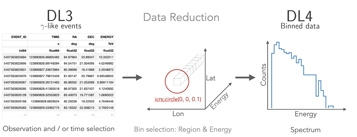
How to compute a 1D spectrum

Gammapy lets you create a 1D spectrum by defining an analysis region in the sky and energy binning using RegionGeom object. The events and instrument response are binned into RegionNDMap and IRFMap objects. In addition you can choose to estimate the background from data using e.g. a reflected regions method. Flux points can be computed using the FluxPointsEstimator.

1D analysis tutorial 1D analysis tutorial with point-like IRFs 1D analysis tutorial of extended sources

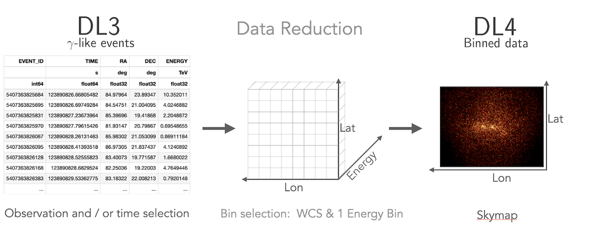
How to compute a 2D image

Gammapy treats 2D maps as 3D cubes with one bin in energy. Computation of 2D images can be done following a 3D analysis with one bin with a fixed spectral index, or following the classical ring background estimation.

2D analysis tutorial 2D analysis tutorial with ring background

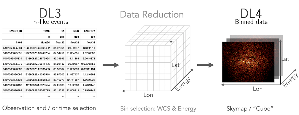
How to compute a 3D cube

Gammapy lets you perform a combined spectral and spatial analysis as well. This is sometimes called in jargon a “cube analysis”. Based on the 3D data reduction Gammapy can also simulate events. Flux points can be computed using the FluxPointsEstimator.

3D analysis tutorial 3D analysis tutorial with event sampling

How to compute a lightcurve

Gammapy allows you to compute light curves in various ways. Light curves can be computed for a 1D or 3D analysis scenario (see above) by either grouping or splitting the DL3 data into multiple time intervals. Grouping multiple observations allows for computing e.g. monthly or nightly binned light curves, while splitting of a single observation allows to compute light curves for flares. You can also compute light curves in multiple energy bands. In all cases the light curve is computed using the LightCurveEstimator.

Light curve tutorial Light curve tutorial for flares

How to combine data from multiple instruments

Gammapy offers the possibility to combine data from multiple instruments in a “joint-likelihood” fit. This can be done at multiple data levels and independent dimensionality of the data. Gammapy can handle 1D and 3D datasets at the same time and can also include e.g. flux points in a combined likelihood fit.

Combined 1D / 3D analysis tutorial SED fitting tutorial