Spectral analysis

Perform a full region based on-off spectral analysis and fit the resulting datasets.

Prerequisites

• Understanding how spectral extraction is performed in Cherenkov astronomy, in particular regarding OFF background measurements.

• Understanding the basics data reduction and modeling/fitting process with the gammapy library API as shown in the Low level API tutorial.

Context

While 3D analyses allow in principle to consider complex field of views containing overlapping gamma-ray sources, in many cases we might have an observation with a single, strong, point-like source in the field of view. A spectral analysis, in that case, might consider all the events inside a source (or ON) region and bin them in energy only, obtaining 1D datasets.

In classical Cherenkov astronomy, the background estimation technique associated with this method measures the number of events in OFF regions taken in regions of the field-of-view devoid of gamma-ray emitters, where the background rate is assumed to be equal to the one in the ON region.

This allows to use a specific fit statistics for ON-OFF measurements, the wstat (see wstat), where no background model is assumed. Background is treated as a set of nuisance parameters. This removes some systematic effects connected to the choice or the quality of the background model. But this comes at the expense of larger statistical uncertainties on the fitted model parameters.

Objective: perform a full region based spectral analysis of 4 Crab observations of H.E.S.S. data release 1 and fit the resulting datasets.

Introduction

Here, as usual, we use the DataStore to retrieve a list of selected observations (Observations). Then, we define the ON region containing the source and the geometry of the SpectrumDataset object we want to produce. We then create the corresponding dataset Maker.

We have to define the Maker object that will extract the OFF counts from reflected regions in the field-of-view. To ensure we use data in an energy range where the quality of the IRFs is good enough we also create a safe range Maker.

We can then proceed with data reduction with a loop over all selected observations to produce datasets in the relevant geometry.

We can then explore the resulting datasets and look at the cumulative signal and significance of our source. We finally proceed with model fitting.

In practice, we have to:

• Create a DataStore pointing to the relevant data

• Apply an observation selection to produce a list of observations, a Observations object.

• Define a geometry of the spectrum we want to produce:

  • Create a CircleSkyRegion for the ON extraction region

  • Create a MapAxis for the energy binnings: one for the reconstructed (i.e.measured) energy, the other for the true energy (i.e.the one used by IRFs and models)

• Create the necessary makers :

  • the spectrum dataset maker : SpectrumDatasetMaker - the OFF background maker, here a ReflectedRegionsBackgroundMaker

  • and the safe range maker : SafeMaskMaker

• Perform the data reduction loop. And for every observation:

  • Apply the makers sequentially to produce a SpectrumDatasetOnOff

  • Append it to list of datasets

• Define the SkyModel to apply to the dataset.

• Create a Fit object and run it to fit the model parameters

• Apply a FluxPointsEstimator to compute flux points for the spectral part of the fit.

from pathlib import Path

# Check package versions
import astropy.units as u
from astropy.coordinates import Angle, SkyCoord
from regions import CircleSkyRegion

# %matplotlib inline
import matplotlib.pyplot as plt

Setup

As usual, we’ll start with some setup …

from IPython.display import display
from gammapy.data import DataStore
from gammapy.datasets import (
    Datasets,
    FluxPointsDataset,
    SpectrumDataset,
    SpectrumDatasetOnOff,
)
from gammapy.estimators import FluxPointsEstimator
from gammapy.estimators.utils import resample_energy_edges
from gammapy.makers import (
    ReflectedRegionsBackgroundMaker,
    SafeMaskMaker,
    SpectrumDatasetMaker,
)
from gammapy.maps import MapAxis, RegionGeom, WcsGeom
from gammapy.modeling import Fit
from gammapy.modeling.models import (
    ExpCutoffPowerLawSpectralModel,
    SkyModel,
    create_crab_spectral_model,
)

Check setup

from gammapy.utils.check import check_tutorials_setup
from gammapy.visualization import plot_spectrum_datasets_off_regions

check_tutorials_setup()

System:

        python_executable      : /home/runner/work/gammapy-docs/gammapy-docs/gammapy/.tox/build_docs/bin/python
        python_version         : 3.9.20
        machine                : x86_64
        system                 : Linux


Gammapy package:

        version                : 2.0.dev2+g10bce85c9
        path                   : /home/runner/work/gammapy-docs/gammapy-docs/gammapy/.tox/build_docs/lib/python3.9/site-packages/gammapy


Other packages:

        numpy                  : 1.26.4
        scipy                  : 1.13.1
        astropy                : 5.2.2
        regions                : 0.8
        click                  : 8.1.7
        yaml                   : 6.0.2
        IPython                : 8.18.1
        jupyterlab             : not installed
        matplotlib             : 3.9.2
        pandas                 : not installed
        healpy                 : 1.17.3
        iminuit                : 2.30.1
        sherpa                 : 4.16.1
        naima                  : 0.10.0
        emcee                  : 3.1.6
        corner                 : 2.2.2
        ray                    : 2.38.0


Gammapy environment variables:

        GAMMAPY_DATA           : /home/runner/work/gammapy-docs/gammapy-docs/gammapy-datasets/dev

Load Data

First, we select and load some H.E.S.S. observations of the Crab nebula.

We will access the events, effective area, energy dispersion, livetime and PSF for containment correction.

datastore = DataStore.from_dir("$GAMMAPY_DATA/hess-dl3-dr1/")
obs_ids = [23523, 23526, 23559, 23592]
observations = datastore.get_observations(obs_ids)

Define Target Region

The next step is to define a signal extraction region, also known as on region. In the simplest case this is just a CircleSkyRegion.

target_position = SkyCoord(ra=83.63, dec=22.01, unit="deg", frame="icrs")
on_region_radius = Angle("0.11 deg")
on_region = CircleSkyRegion(center=target_position, radius=on_region_radius)

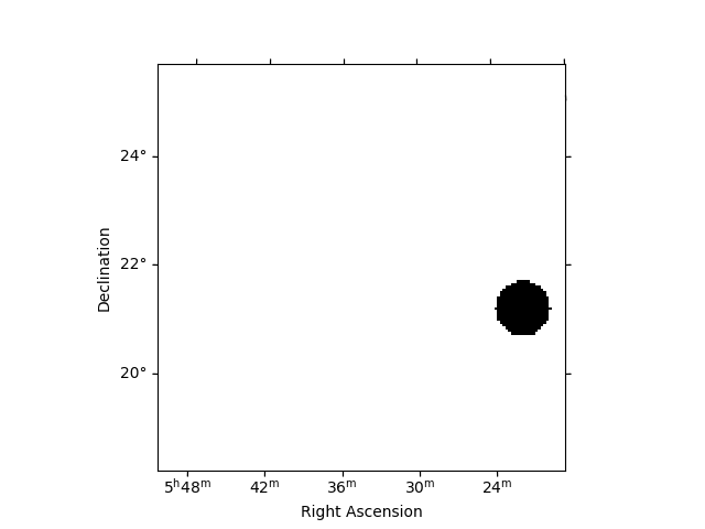
Create exclusion mask

We will use the reflected regions method to place off regions to estimate the background level in the on region. To make sure the off regions don’t contain gamma-ray emission, we create an exclusion mask.

Using http://gamma-sky.net/ we find that there’s only one known gamma-ray source near the Crab nebula: the AGN called RGB J0521+212 at GLON = 183.604 deg and GLAT = -8.708 deg.

exclusion_region = CircleSkyRegion(
    center=SkyCoord(183.604, -8.708, unit="deg", frame="galactic"),
    radius=0.5 * u.deg,
)

skydir = target_position.galactic
geom = WcsGeom.create(
    npix=(150, 150), binsz=0.05, skydir=skydir, proj="TAN", frame="icrs"
)

exclusion_mask = ~geom.region_mask([exclusion_region])
exclusion_mask.plot()
plt.show()

Run data reduction chain

We begin with the configuration of the maker classes:

energy_axis = MapAxis.from_energy_bounds(
    0.1, 40, nbin=10, per_decade=True, unit="TeV", name="energy"
)
energy_axis_true = MapAxis.from_energy_bounds(
    0.05, 100, nbin=20, per_decade=True, unit="TeV", name="energy_true"
)

geom = RegionGeom.create(region=on_region, axes=[energy_axis])
dataset_empty = SpectrumDataset.create(geom=geom, energy_axis_true=energy_axis_true)

dataset_maker = SpectrumDatasetMaker(
    containment_correction=True, selection=["counts", "exposure", "edisp"]
)
bkg_maker = ReflectedRegionsBackgroundMaker(exclusion_mask=exclusion_mask)
safe_mask_maker = SafeMaskMaker(methods=["aeff-max"], aeff_percent=10)

datasets = Datasets()

for obs_id, observation in zip(obs_ids, observations):
    dataset = dataset_maker.run(dataset_empty.copy(name=str(obs_id)), observation)
    dataset_on_off = bkg_maker.run(dataset, observation)
    dataset_on_off = safe_mask_maker.run(dataset_on_off, observation)
    datasets.append(dataset_on_off)

print(datasets)

Datasets
--------

Dataset 0:

  Type       : SpectrumDatasetOnOff
  Name       : 23523
  Instrument : HESS
  Models     :

Dataset 1:

  Type       : SpectrumDatasetOnOff
  Name       : 23526
  Instrument : HESS
  Models     :

Dataset 2:

  Type       : SpectrumDatasetOnOff
  Name       : 23559
  Instrument : HESS
  Models     :

Dataset 3:

  Type       : SpectrumDatasetOnOff
  Name       : 23592
  Instrument : HESS
  Models     :

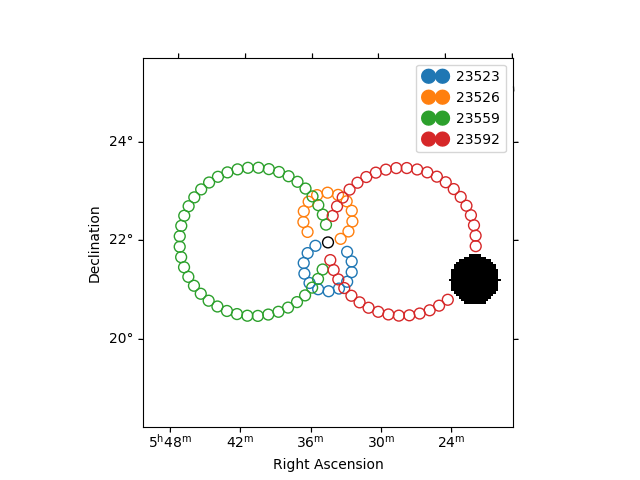
Plot off regions

plt.figure()
ax = exclusion_mask.plot()
on_region.to_pixel(ax.wcs).plot(ax=ax, edgecolor="k")
plot_spectrum_datasets_off_regions(ax=ax, datasets=datasets)
plt.show()

/home/runner/work/gammapy-docs/gammapy-docs/gammapy/.tox/build_docs/lib/python3.9/site-packages/regions/shapes/circle.py:161: UserWarning: Setting the 'color' property will override the edgecolor or facecolor properties.
  return Circle(xy=xy, radius=radius, **mpl_kwargs)
/home/runner/work/gammapy-docs/gammapy-docs/gammapy/.tox/build_docs/lib/python3.9/site-packages/gammapy/visualization/datasets.py:84: UserWarning: Setting the 'color' property will override the edgecolor or facecolor properties.
  handle = Patch(**plot_kwargs)

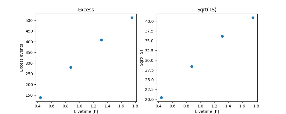
Source statistic

Next we’re going to look at the overall source statistics in our signal region.

info_table = datasets.info_table(cumulative=True)

display(info_table)

  name  counts       excess      ...   acceptance_off          alpha
                                 ...
------- ------ ----------------- ... ------------------ -------------------
stacked    149            139.25 ...              216.0  0.0833333358168602
stacked    303            280.75 ... 443.99993896484375  0.0833333432674408
stacked    439 408.7743835449219 ...  1100.523681640625 0.05088486522436142
stacked    550  512.135498046875 ... 1698.3189697265625 0.04357249662280083

And make the corresponding plots

fig, (ax_excess, ax_sqrt_ts) = plt.subplots(figsize=(10, 4), ncols=2, nrows=1)
ax_excess.plot(
    info_table["livetime"].to("h"),
    info_table["excess"],
    marker="o",
    ls="none",
)

ax_excess.set_title("Excess")
ax_excess.set_xlabel("Livetime [h]")
ax_excess.set_ylabel("Excess events")

ax_sqrt_ts.plot(
    info_table["livetime"].to("h"),
    info_table["sqrt_ts"],
    marker="o",
    ls="none",
)

ax_sqrt_ts.set_title("Sqrt(TS)")
ax_sqrt_ts.set_xlabel("Livetime [h]")
ax_sqrt_ts.set_ylabel("Sqrt(TS)")
plt.show()

Finally you can write the extracted datasets to disk using the OGIP format (PHA, ARF, RMF, BKG, see here for details):

path = Path("spectrum_analysis")
path.mkdir(exist_ok=True)

for dataset in datasets:
    dataset.write(filename=path / f"obs_{dataset.name}.fits.gz", overwrite=True)

If you want to read back the datasets from disk you can use:

datasets = Datasets()

for obs_id in obs_ids:
    filename = path / f"obs_{obs_id}.fits.gz"
    datasets.append(SpectrumDatasetOnOff.read(filename))

Fit spectrum

Now we’ll fit a global model to the spectrum. First we do a joint likelihood fit to all observations. If you want to stack the observations see below. We will also produce a debug plot in order to show how the global fit matches one of the individual observations.

spectral_model = ExpCutoffPowerLawSpectralModel(
    amplitude=1e-12 * u.Unit("cm-2 s-1 TeV-1"),
    index=2,
    lambda_=0.1 * u.Unit("TeV-1"),
    reference=1 * u.TeV,
)
model = SkyModel(spectral_model=spectral_model, name="crab")

datasets.models = [model]

fit_joint = Fit()
result_joint = fit_joint.run(datasets=datasets)

# we make a copy here to compare it later
model_best_joint = model.copy()

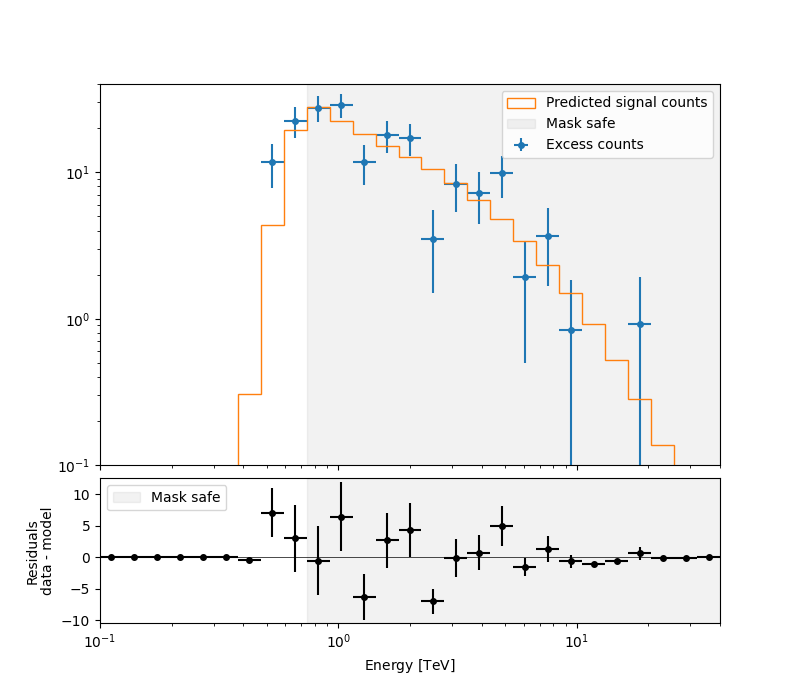
Fit quality and model residuals

We can access the results dictionary to see if the fit converged:

print(result_joint)

OptimizeResult

        backend    : minuit
        method     : migrad
        success    : True
        message    : Optimization terminated successfully.
        nfev       : 244
        total stat : 86.12

CovarianceResult

        backend    : minuit
        method     : hesse
        success    : True
        message    : Hesse terminated successfully.

and check the best-fit parameters

display(result_joint.models.to_parameters_table())

model type    name     value         unit      ... min max frozen link prior
----- ---- --------- ---------- -------------- ... --- --- ------ ---- -----
 crab          index 2.2727e+00                ... nan nan  False
 crab      amplitude 4.7913e-11 cm-2 s-1 TeV-1 ... nan nan  False
 crab      reference 1.0000e+00            TeV ... nan nan   True
 crab        lambda_ 1.2097e-01          TeV-1 ... nan nan  False
 crab          alpha 1.0000e+00                ... nan nan   True

A simple way to inspect the model residuals is using the function plot_fit()

ax_spectrum, ax_residuals = datasets[0].plot_fit()
ax_spectrum.set_ylim(0.1, 40)
plt.show()

For more ways of assessing fit quality, please refer to the dedicated Fitting tutorial.

Compute Flux Points

To round up our analysis we can compute flux points by fitting the norm of the global model in energy bands. We create an instance of the FluxPointsEstimator, by passing the dataset and the energy binning:

fpe = FluxPointsEstimator(
    energy_edges=energy_axis.edges, source="crab", selection_optional="all"
)
flux_points = fpe.run(datasets=datasets)

Here is a the table of the resulting flux points:

display(flux_points.to_table(sed_type="dnde", formatted=True))

e_ref  e_min  e_max        dnde      ...    counts    success   norm_scan
 TeV    TeV    TeV   1 / (cm2 s TeV) ...
------ ------ ------ --------------- ... ------------ ------- --------------
 0.112  0.100  0.125             nan ...   0.0 .. 0.0   False 0.200 .. 5.000
 0.139  0.125  0.156             nan ...   0.0 .. 0.0   False 0.200 .. 5.000
 0.174  0.156  0.195             nan ...   0.0 .. 0.0   False 0.200 .. 5.000
 0.217  0.195  0.243             nan ...   0.0 .. 0.0   False 0.200 .. 5.000
 0.271  0.243  0.303             nan ...   0.0 .. 0.0   False 0.200 .. 5.000
 0.339  0.303  0.379             nan ...   0.0 .. 0.0   False 0.200 .. 5.000
 0.423  0.379  0.473             nan ...   0.0 .. 0.0   False 0.200 .. 5.000
 0.528  0.473  0.590             nan ...   0.0 .. 0.0   False 0.200 .. 5.000
 0.659  0.590  0.737       1.132e-10 ...   0.0 .. 0.0    True 0.200 .. 5.000
 0.823  0.737  0.920       6.950e-11 ... 30.0 .. 25.0    True 0.200 .. 5.000
   ...    ...    ...             ... ...          ...     ...            ...
 4.859  4.348  5.429       7.435e-13 ...  10.0 .. 3.0    True 0.200 .. 5.000
 6.066  5.429  6.778       3.779e-13 ...   2.0 .. 3.0    True 0.200 .. 5.000
 7.573  6.778  8.462       2.240e-13 ...   4.0 .. 1.0    True 0.200 .. 5.000
 9.454  8.462 10.564       1.190e-13 ...   1.0 .. 4.0    True 0.200 .. 5.000
11.803 10.564 13.189       5.214e-14 ...   0.0 .. 0.0    True 0.200 .. 5.000
14.736 13.189 16.465       7.642e-15 ...   0.0 .. 0.0    True 0.200 .. 5.000
18.397 16.465 20.556       1.494e-14 ...   1.0 .. 0.0    True 0.200 .. 5.000
22.968 20.556 25.663      -5.332e-31 ...   0.0 .. 0.0    True 0.200 .. 5.000
28.675 25.663 32.040       7.267e-23 ...   0.0 .. 0.0    True 0.200 .. 5.000
35.799 32.040 40.000      -4.119e-32 ...   0.0 .. 0.0    True 0.200 .. 5.000
Length = 27 rows

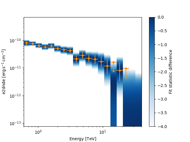
Now we plot the flux points and their likelihood profiles. For the plotting of upper limits we choose a threshold of TS < 4.

fig, ax = plt.subplots()
flux_points.plot(ax=ax, sed_type="e2dnde", color="darkorange")
flux_points.plot_ts_profiles(ax=ax, sed_type="e2dnde")
ax.set_xlim(0.6, 40)
plt.show()

Note: it is also possible to plot the flux distribution with the spectral model overlaid, but you must ensure the axis binning is identical for the flux points and integral flux.

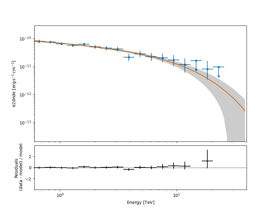
The final plot with the best fit model, flux points and residuals can be quickly made like this:

flux_points_dataset = FluxPointsDataset(
    data=flux_points, models=model_best_joint.copy()
)
ax, _ = flux_points_dataset.plot_fit()
ax.set_xlim(0.6, 40)
plt.show()

Stack observations

An alternative approach to fitting the spectrum is stacking all observations first and the fitting a model. For this we first stack the individual datasets:

dataset_stacked = Datasets(datasets).stack_reduce()

Again we set the model on the dataset we would like to fit (in this case it’s only a single one) and pass it to the Fit object:

dataset_stacked.models = model
stacked_fit = Fit()
result_stacked = stacked_fit.run([dataset_stacked])

# Make a copy to compare later
model_best_stacked = model.copy()

print(result_stacked)

OptimizeResult

        backend    : minuit
        method     : migrad
        success    : True
        message    : Optimization terminated successfully.
        nfev       : 54
        total stat : 8.16

CovarianceResult

        backend    : minuit
        method     : hesse
        success    : True
        message    : Hesse terminated successfully.

And display the parameter table

display(model_best_joint.parameters.to_table())

display(model_best_stacked.parameters.to_table())

type    name     value         unit        error   min max frozen link prior
---- --------- ---------- -------------- --------- --- --- ------ ---- -----
         index 2.2727e+00                1.566e-01 nan nan  False
     amplitude 4.7913e-11 cm-2 s-1 TeV-1 3.600e-12 nan nan  False
     reference 1.0000e+00            TeV 0.000e+00 nan nan   True
       lambda_ 1.2097e-01          TeV-1 5.382e-02 nan nan  False
         alpha 1.0000e+00                0.000e+00 nan nan   True
type    name     value         unit        error   min max frozen link prior
---- --------- ---------- -------------- --------- --- --- ------ ---- -----
         index 2.2785e+00                1.563e-01 nan nan  False
     amplitude 4.7800e-11 cm-2 s-1 TeV-1 3.566e-12 nan nan  False
     reference 1.0000e+00            TeV 0.000e+00 nan nan   True
       lambda_ 1.1830e-01          TeV-1 5.329e-02 nan nan  False
         alpha 1.0000e+00                0.000e+00 nan nan   True

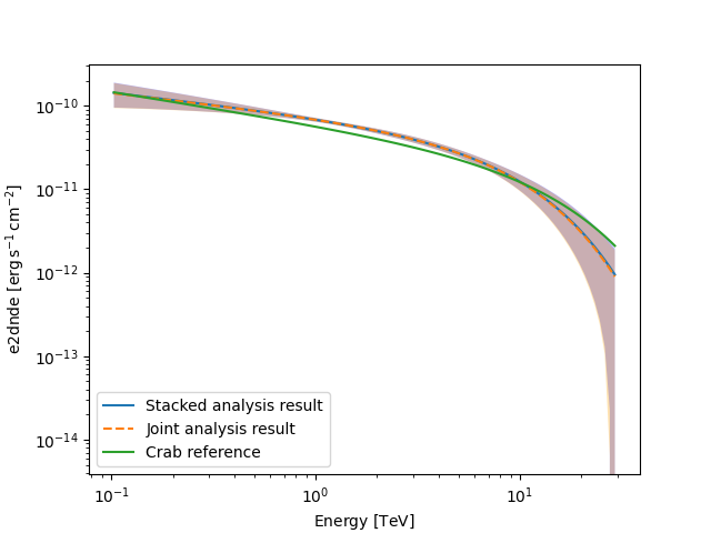
Finally, we compare the results of our stacked analysis to a previously published Crab Nebula Spectrum for reference. This is available in create_crab_spectral_model.

fig, ax = plt.subplots()

plot_kwargs = {
    "energy_bounds": [0.1, 30] * u.TeV,
    "sed_type": "e2dnde",
    "yunits": u.Unit("erg cm-2 s-1"),
    "ax": ax,
}

# plot stacked model
model_best_stacked.spectral_model.plot(**plot_kwargs, label="Stacked analysis result")
model_best_stacked.spectral_model.plot_error(facecolor="blue", alpha=0.3, **plot_kwargs)

# plot joint model
model_best_joint.spectral_model.plot(
    **plot_kwargs, label="Joint analysis result", ls="--"
)
model_best_joint.spectral_model.plot_error(facecolor="orange", alpha=0.3, **plot_kwargs)

create_crab_spectral_model("hess_ecpl").plot(
    **plot_kwargs,
    label="Crab reference",
)
ax.legend()
plt.show()

# sphinx_gallery_thumbnail_number = 5

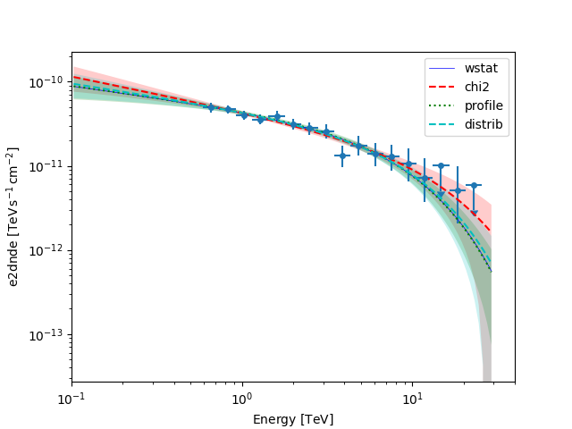
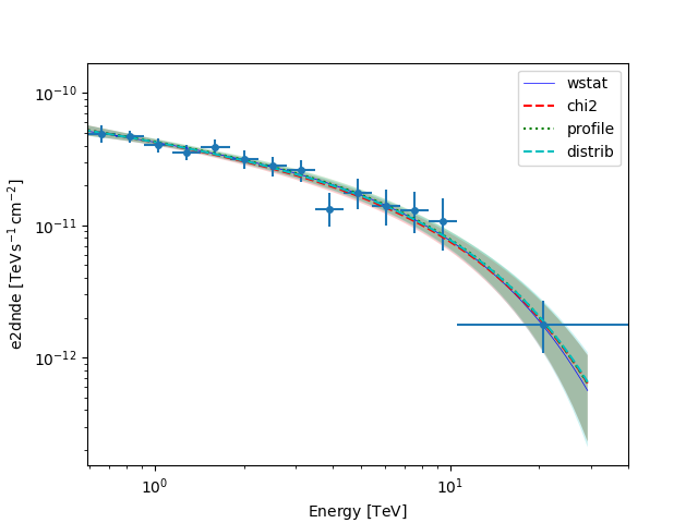
A note on statistics

Different statistic are available for the FluxPointsDataset :

• chi2 : estimate from chi2 statistics.

• profile : estimate from interpolation of the likelihood profile.

• distribestimate from probability distributions,

  assuming that flux points correspond to asymmetric gaussians and upper limits complementary error functions.

Default is chi2, in that case upper limits are ignored and the mean of asymetrics error is used. So it is recommended to use profile if stat_scan is available on flux points. The distrib case provides an approximation if the profile is not available which allows to take into accounts upper limit and asymetrics error.

In the example below we can see that the profile case matches exactly the result from the joint analysis of the ON/OFF datasets using wstat (as labelled).

def plot_stat(fp_dataset):
    fig, ax = plt.subplots()

    plot_kwargs = {
        "energy_bounds": [0.1, 30] * u.TeV,
        "sed_type": "e2dnde",
        "ax": ax,
    }

    fp_dataset.data.plot(energy_power=2, ax=ax)
    model_best_joint.spectral_model.plot(
        color="b", lw=0.5, **plot_kwargs, label="wstat"
    )

    stat_types = ["chi2", "profile", "distrib"]
    colors = ["red", "g", "c"]
    lss = ["--", ":", "--"]

    for ks, stat in enumerate(stat_types):
        fp_dataset.stat_type = stat

        fit = Fit()
        fit.run([fp_dataset])

        fp_dataset.models[0].spectral_model.plot(
            color=colors[ks], ls=lss[ks], **plot_kwargs, label=stat
        )
        fp_dataset.models[0].spectral_model.plot_error(
            facecolor=colors[ks], **plot_kwargs
        )
        plt.legend()


plot_stat(flux_points_dataset)

In order to avoid discrepancies due to the treatment of upper limits we can utilise the resample_energy_edges for defining energy bins in which the minimum number of sqrt_ts is 2. In that case all the statistics definitions give equivalent results.

energy_edges = resample_energy_edges(dataset_stacked, conditions={"sqrt_ts_min": 2})

fpe_no_ul = FluxPointsEstimator(
    energy_edges=energy_edges, source="crab", selection_optional="all"
)
flux_points_no_ul = fpe_no_ul.run(datasets=datasets)
flux_points_dataset_no_ul = FluxPointsDataset(
    data=flux_points_no_ul,
    models=model_best_joint.copy(),
)

plot_stat(flux_points_dataset_no_ul)

Exercises

Now you have learned the basics of a spectral analysis with Gammapy. To practice you can continue with the following exercises:

• Fit a different spectral model to the data. You could try ExpCutoffPowerLawSpectralModel or LogParabolaSpectralModel.

• Compute flux points for the stacked dataset.

• Create a FluxPointsDataset with the flux points you have computed for the stacked dataset and fit the flux points again with obe of the spectral models. How does the result compare to the best fit model, that was directly fitted to the counts data?

What next?

The methods shown in this tutorial is valid for point-like or midly extended sources where we can assume that the IRF taken at the region center is valid over the whole region. If one wants to extract the 1D spectrum of a large source and properly average the response over the extraction region, one has to use a different approach explained in the Spectral analysis of extended sources tutorial.