Note
Go to the end to download the full example code or to run this example in your browser via Binder.
3D detailed analysis#
Perform detailed 3D stacked and joint analysis.
This tutorial does a 3D map based analysis on the galactic center, using simulated observations from the CTA-1DC. We will use the high level interface for the data reduction, and then do a detailed modelling. This will be done in two different ways:
stacking all the maps together and fitting the stacked maps
handling all the observations separately and doing a joint fitting on all the maps
from pathlib import Path
import astropy.units as u
from regions import CircleSkyRegion

# %matplotlib inline
import matplotlib.pyplot as plt
from IPython.display import display
from gammapy.analysis import Analysis, AnalysisConfig
from gammapy.estimators import ExcessMapEstimator
from gammapy.modeling import Fit
from gammapy.modeling.models import (
    ExpCutoffPowerLawSpectralModel,
    FoVBackgroundModel,
    Models,
    PointSpatialModel,
    SkyModel,
)
from gammapy.visualization import plot_distribution
Analysis configuration#
In this section we select observations and define the analysis geometries, irrespective of joint/stacked analysis. For configuration of the analysis, we will programmatically build a config file from scratch.
config = AnalysisConfig()
# The config file is now empty, with only a few defaults specified.
print(config)

# Selecting the observations
config.observations.datastore = "$GAMMAPY_DATA/cta-1dc/index/gps/"
config.observations.obs_ids = [110380, 111140, 111159]

# Defining a reference geometry for the reduced datasets

config.datasets.type = "3d"  # Analysis type is 3D

config.datasets.geom.wcs.skydir = {
    "lon": "0 deg",
    "lat": "0 deg",
    "frame": "galactic",
}  # The WCS geometry - centered on the galactic center
config.datasets.geom.wcs.width = {"width": "10 deg", "height": "8 deg"}
config.datasets.geom.wcs.binsize = "0.02 deg"

# Cutout size (for the run-wise event selection)
config.datasets.geom.selection.offset_max = 3.5 * u.deg
config.datasets.safe_mask.methods = ["aeff-default", "offset-max"]

# We now fix the energy axis for the counts map - (the reconstructed energy binning)
config.datasets.geom.axes.energy.min = "0.1 TeV"
config.datasets.geom.axes.energy.max = "10 TeV"
config.datasets.geom.axes.energy.nbins = 10

# We now fix the energy axis for the IRF maps (exposure, etc) - (the true energy binning)
config.datasets.geom.axes.energy_true.min = "0.08 TeV"
config.datasets.geom.axes.energy_true.max = "12 TeV"
config.datasets.geom.axes.energy_true.nbins = 14

print(config)
AnalysisConfig

    general:
        log:
            level: info
            filename: null
            filemode: null
            format: null
            datefmt: null
        outdir: .
        n_jobs: 1
        datasets_file: null
        models_file: null
    observations:
        datastore: /home/runner/work/gammapy-docs/gammapy-docs/gammapy-datasets/dev/hess-dl3-dr1
        obs_ids: []
        obs_file: null
        obs_cone:
            frame: null
            lon: null
            lat: null
            radius: null
        obs_time:
            start: null
            stop: null
        required_irf:
        - aeff
        - edisp
        - psf
        - bkg
    datasets:
        type: 1d
        stack: true
        geom:
            wcs:
                skydir:
                    frame: null
                    lon: null
                    lat: null
                binsize: 0.02 deg
                width:
                    width: 5.0 deg
                    height: 5.0 deg
                binsize_irf: 0.2 deg
            selection:
                offset_max: 2.5 deg
            axes:
                energy:
                    min: 1.0 TeV
                    max: 10.0 TeV
                    nbins: 5
                energy_true:
                    min: 0.5 TeV
                    max: 20.0 TeV
                    nbins: 16
        map_selection:
        - counts
        - exposure
        - background
        - psf
        - edisp
        background:
            method: null
            exclusion: null
            parameters: {}
        safe_mask:
            methods:
            - aeff-default
            parameters: {}
        on_region:
            frame: null
            lon: null
            lat: null
            radius: null
        containment_correction: true
    fit:
        fit_range:
            min: null
            max: null
    flux_points:
        energy:
            min: null
            max: null
            nbins: null
        source: source
        parameters:
            selection_optional: all
    excess_map:
        correlation_radius: 0.1 deg
        parameters: {}
        energy_edges:
            min: null
            max: null
            nbins: null
    light_curve:
        time_intervals:
            start: null
            stop: null
        energy_edges:
            min: null
            max: null
            nbins: null
        source: source
        parameters:
            selection_optional: all
    metadata:
        creator: Gammapy 2.0.dev4000+g6ed4106cb
        date: '2026-07-21T07:42:37.307819'
        origin: null

AnalysisConfig

    general:
        log:
            level: info
            filename: null
            filemode: null
            format: null
            datefmt: null
        outdir: .
        n_jobs: 1
        datasets_file: null
        models_file: null
    observations:
        datastore: /home/runner/work/gammapy-docs/gammapy-docs/gammapy-datasets/dev/cta-1dc/index/gps
        obs_ids:
        - 110380
        - 111140
        - 111159
        obs_file: null
        obs_cone:
            frame: null
            lon: null
            lat: null
            radius: null
        obs_time:
            start: null
            stop: null
        required_irf:
        - aeff
        - edisp
        - psf
        - bkg
    datasets:
        type: 3d
        stack: true
        geom:
            wcs:
                skydir:
                    frame: galactic
                    lon: 0.0 deg
                    lat: 0.0 deg
                binsize: 0.02 deg
                width:
                    width: 10.0 deg
                    height: 8.0 deg
                binsize_irf: 0.2 deg
            selection:
                offset_max: 3.5 deg
            axes:
                energy:
                    min: 0.1 TeV
                    max: 10.0 TeV
                    nbins: 10
                energy_true:
                    min: 0.08 TeV
                    max: 12.0 TeV
                    nbins: 14
        map_selection:
        - counts
        - exposure
        - background
        - psf
        - edisp
        background:
            method: null
            exclusion: null
            parameters: {}
        safe_mask:
            methods:
            - aeff-default
            - offset-max
            parameters: {}
        on_region:
            frame: null
            lon: null
            lat: null
            radius: null
        containment_correction: true
    fit:
        fit_range:
            min: null
            max: null
    flux_points:
        energy:
            min: null
            max: null
            nbins: null
        source: source
        parameters:
            selection_optional: all
    excess_map:
        correlation_radius: 0.1 deg
        parameters: {}
        energy_edges:
            min: null
            max: null
            nbins: null
    light_curve:
        time_intervals:
            start: null
            stop: null
        energy_edges:
            min: null
            max: null
            nbins: null
        source: source
        parameters:
            selection_optional: all
    metadata:
        creator: Gammapy 2.0.dev4000+g6ed4106cb
        date: '2026-07-21T07:42:37.312580'
        origin: null
Configuration for stacked and joint analysis#
This is done just by specifying the flag on config.datasets.stack.
Since the internal machinery will work differently for the two cases, we
will write it as two config files and save it to disc in YAML format for
future reference.
config_stack = config.model_copy(deep=True)
config_stack.datasets.stack = True

config_joint = config.model_copy(deep=True)
config_joint.datasets.stack = False

# To prevent unnecessary cluttering, we write it in a separate folder.
path = Path("analysis_3d")
path.mkdir(exist_ok=True)
config_joint.write(path=path / "config_joint.yaml", overwrite=True)
config_stack.write(path=path / "config_stack.yaml", overwrite=True)
Stacked analysis#
Data reduction#
We first show the steps for the stacked analysis and then repeat the same for the joint analysis later
# Reading yaml file:
config_stacked = AnalysisConfig.read(path=path / "config_stack.yaml")

analysis_stacked = Analysis(config_stacked)

# select observations:
analysis_stacked.get_observations()

# run data reduction
analysis_stacked.get_datasets()
/home/runner/work/gammapy-docs/gammapy-docs/gammapy/.tox/build_docs/lib/python3.12/site-packages/astropy/units/core.py:2102: UnitsWarning: '1/s/MeV/sr' did not parse as fits unit: Numeric factor not supported by FITS If this is meant to be a custom unit, define it with 'u.def_unit'. To have it recognized inside a file reader or other code, enable it with 'u.add_enabled_units'. For details, see https://docs.astropy.org/en/latest/units/combining_and_defining.html
  warnings.warn(msg, UnitsWarning)
We have one final dataset, which we can print and explore
dataset_stacked = analysis_stacked.datasets["stacked"]
print(dataset_stacked)
MapDataset
----------

  Name                            : stacked

  Total counts                    : 121241
  Total background counts         : 108043.52
  Total excess counts             : 13197.48

  Predicted counts                : 108043.52
  Predicted background counts     : 108043.52
  Predicted excess counts         : nan

  Exposure min                    : 6.28e+07 m2 s
  Exposure max                    : 1.90e+10 m2 s

  Number of total bins            : 2000000
  Number of fit bins              : 1411180

  Fit statistic type              : cash
  Fit statistic value (-2 log(L)) : nan

  Number of models                : 0
  Number of parameters            : 0
  Number of free parameters       : 0
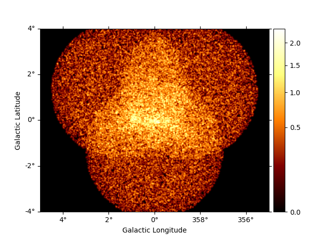
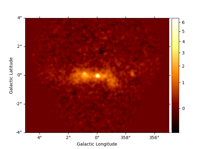
To visualise a counts map in different energy slices, you can use the
plot_grid or plot_interactive
functionalities, or create a plot of the counts summed over the energy axis:
dataset_stacked.counts.sum_over_axes().smooth(0.02 * u.deg).plot(add_cbar=True)
plt.show()
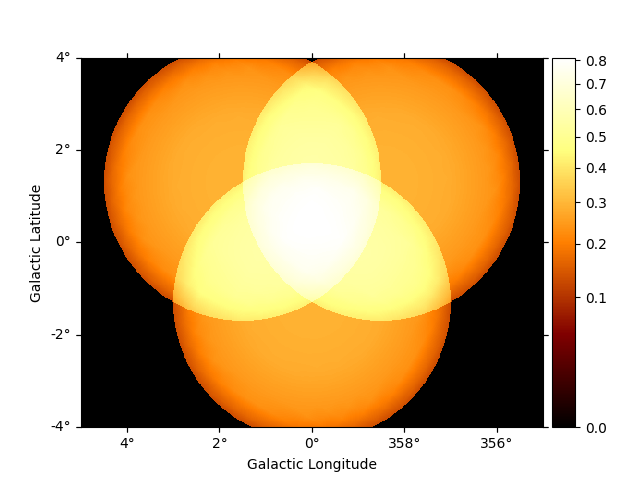
Similarly with the background map:
dataset_stacked.background.sum_over_axes().plot(add_cbar=True)
plt.show()
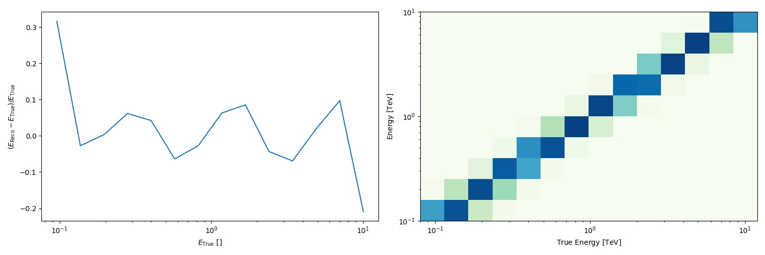
We can quickly check the PSF
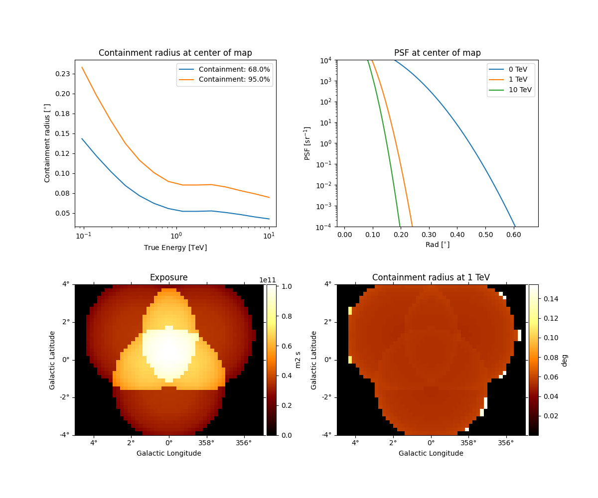
And the energy dispersion in the center of the map
You can also get an excess image with a few lines of code:
excess = dataset_stacked.excess.sum_over_axes()
excess.smooth("0.06 deg").plot(stretch="sqrt", add_cbar=True)
plt.show()
Modeling and fitting#
Now comes the interesting part of the analysis - choosing appropriate models for our source and fitting them.
We choose a point source model with an exponential cutoff power-law spectrum.
To perform the fit on a restricted energy range, we can create a
specific mask. On the dataset, the mask_fit is a Map sharing
the same geometry as the MapDataset and containing boolean data.
To create a mask to limit the fit within a restricted energy range, one
can rely on the energy_mask() method.
For more details on masks and the techniques to create them in gammapy, please checkout the dedicated Mask maps tutorial.
dataset_stacked.mask_fit = dataset_stacked.counts.geom.energy_mask(
    energy_min=0.3 * u.TeV, energy_max=None
)

spatial_model = PointSpatialModel(
    lon_0="-0.05 deg", lat_0="-0.05 deg", frame="galactic"
)
spectral_model = ExpCutoffPowerLawSpectralModel(
    index=2.3,
    amplitude=2.8e-12 * u.Unit("cm-2 s-1 TeV-1"),
    reference=1.0 * u.TeV,
    lambda_=0.02 / u.TeV,
)

model = SkyModel(
    spatial_model=spatial_model,
    spectral_model=spectral_model,
    name="gc-source",
)

bkg_model = FoVBackgroundModel(dataset_name="stacked")
bkg_model.spectral_model.norm.value = 1.3

models_stacked = Models([model, bkg_model])

dataset_stacked.models = models_stacked

fit = Fit(optimize_opts={"print_level": 1})
result = fit.run(datasets=[dataset_stacked])
Fit quality assessment and model residuals for a MapDataset#
We can access the results dictionary to see if the fit converged:
print(result)
OptimizeResult

        backend    : minuit
        method     : migrad
        success    : True
        message    : Optimization terminated successfully.
        nfev       : 192
        total stat : 180458.61

CovarianceResult

        backend    : minuit
        method     : hesse
        success    : True
        message    : Hesse terminated successfully.
Check best-fit parameters and error estimates:
display(models_stacked.to_parameters_table())
   model    type    name      value    ...    max    frozen link prior
----------- ---- --------- ----------- ... --------- ------ ---- -----
  gc-source          index  2.4159e+00 ...       nan  False
  gc-source      amplitude  2.6566e-12 ...       nan  False
  gc-source      reference  1.0000e+00 ...       nan   True
  gc-source        lambda_ -1.4049e-02 ...       nan  False
  gc-source          alpha  1.0000e+00 ...       nan   True
  gc-source          lon_0 -4.8086e-02 ...       nan  False
  gc-source          lat_0 -5.2600e-02 ... 9.000e+01  False
stacked-bkg           tilt  0.0000e+00 ...       nan   True
stacked-bkg           norm  1.3481e+00 ...       nan  False
stacked-bkg      reference  1.0000e+00 ...       nan   True
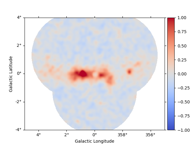
A quick way to inspect the model residuals is using the function
plot_residuals_spatial(). This function computes and
plots a residual image (by default, the smoothing radius is 0.1 deg
and method=diff, which corresponds to a simple data - model
plot):
dataset_stacked.plot_residuals_spatial(method="diff/sqrt(model)", vmin=-1, vmax=1)
plt.show()
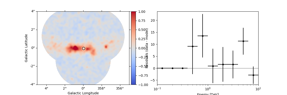
The more general function plot_residuals() can also
extract and display spectral residuals in a region:
region = CircleSkyRegion(spatial_model.position, radius=0.15 * u.deg)
dataset_stacked.plot_residuals(
    kwargs_spatial=dict(method="diff/sqrt(model)", vmin=-1, vmax=1),
    kwargs_spectral=dict(region=region),
)
plt.show()
This way of accessing residuals is quick and handy, but comes with limitations. For example:
In case a fitting energy range was defined using a
mask_fit, it won’t be taken into account. Residuals will be summed up over the whole reconstructed energy rangeIn order to make a proper statistic treatment, instead of simple residuals a proper residuals significance map should be computed
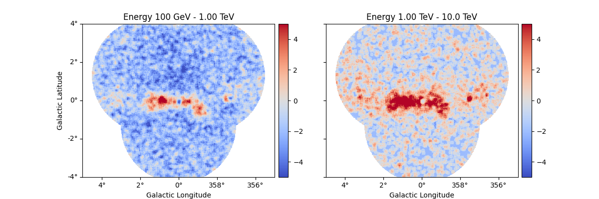
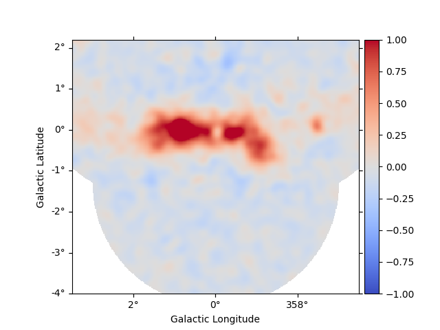
A more accurate way to inspect spatial residuals is the following:
estimator = ExcessMapEstimator(
    correlation_radius="0.1 deg",
    selection_optional=[],
    energy_edges=[0.1, 1, 10] * u.TeV,
)

result = estimator.run(dataset_stacked)
result["sqrt_ts"].plot_grid(
    figsize=(12, 4), cmap="coolwarm", add_cbar=True, vmin=-5, vmax=5, ncols=2
)
plt.show()
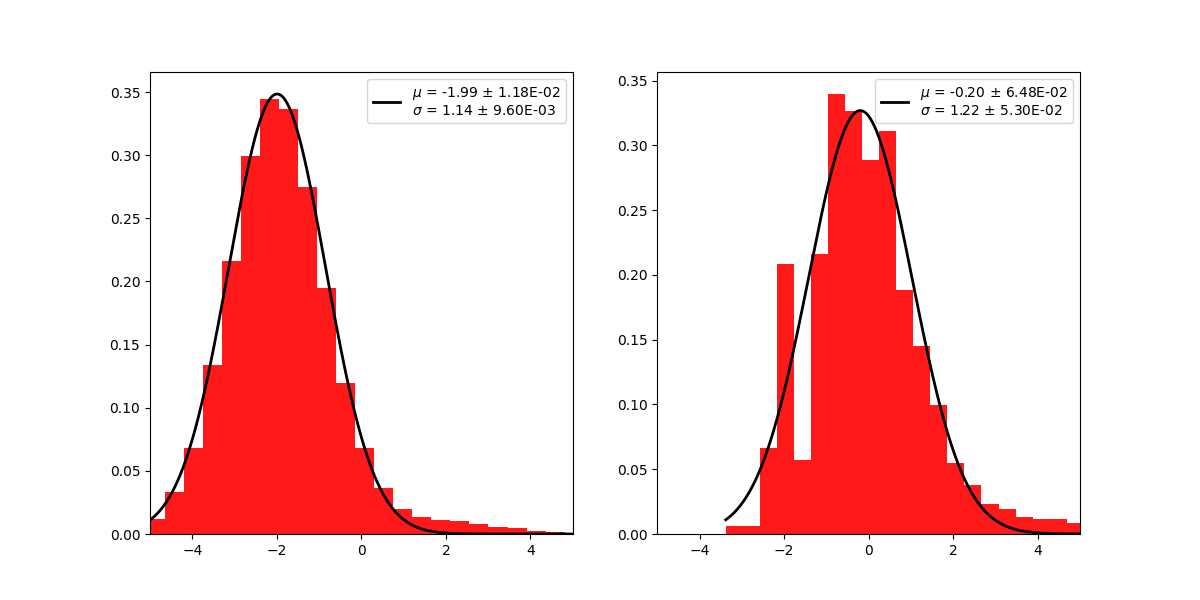
Distribution of residuals significance in the full map geometry:
significance_map = result["sqrt_ts"]

kwargs_hist = {"density": True, "alpha": 0.9, "color": "red", "bins": 40}

ax, res = plot_distribution(
    significance_map,
    func="norm",
    kwargs_hist=kwargs_hist,
    kwargs_axes={"xlim": (-5, 5)},
)

plt.show()
Here we could also plot the number of predicted counts for each model and
for the background in our dataset by using the
plot_npred_signal function.
Joint analysis#
In this section, we perform a joint analysis of the same data. Of course, joint fitting is considerably heavier than stacked one, and should always be handled with care. For brevity, we only show the analysis for a point source fitting without re-adding a diffuse component again.
Data reduction#
# Read the yaml file from disk
config_joint = AnalysisConfig.read(path=path / "config_joint.yaml")
analysis_joint = Analysis(config_joint)

# select observations:
analysis_joint.get_observations()

# run data reduction
analysis_joint.get_datasets()

# You can see there are 3 datasets now
print(analysis_joint.datasets)
/home/runner/work/gammapy-docs/gammapy-docs/gammapy/.tox/build_docs/lib/python3.12/site-packages/astropy/units/core.py:2102: UnitsWarning: '1/s/MeV/sr' did not parse as fits unit: Numeric factor not supported by FITS If this is meant to be a custom unit, define it with 'u.def_unit'. To have it recognized inside a file reader or other code, enable it with 'u.add_enabled_units'. For details, see https://docs.astropy.org/en/latest/units/combining_and_defining.html
  warnings.warn(msg, UnitsWarning)
Datasets
--------

Dataset 0:

  Type       : MapDataset
  Name       : rIa4deAo
  Instrument : CTA
  Models     :

Dataset 1:

  Type       : MapDataset
  Name       : 8WQg1s4H
  Instrument : CTA
  Models     :

Dataset 2:

  Type       : MapDataset
  Name       : cSa_ClGO
  Instrument : CTA
  Models     :
You can access each one by name or by index, eg:
print(analysis_joint.datasets[0])
MapDataset
----------

  Name                            : rIa4deAo

  Total counts                    : 40481
  Total background counts         : 36014.51
  Total excess counts             : 4466.49

  Predicted counts                : 36014.51
  Predicted background counts     : 36014.51
  Predicted excess counts         : nan

  Exposure min                    : 6.28e+07 m2 s
  Exposure max                    : 6.68e+09 m2 s

  Number of total bins            : 1085000
  Number of fit bins              : 693940

  Fit statistic type              : cash
  Fit statistic value (-2 log(L)) : nan

  Number of models                : 0
  Number of parameters            : 0
  Number of free parameters       : 0
After the data reduction stage, it is nice to get a quick summary info
on the datasets. Here, we look at the statistics in the center of Map,
by passing an appropriate region. To get info on the entire spatial
map, omit the region argument.
display(analysis_joint.datasets.info_table())

models_joint = Models()

model_joint = model.copy(name="source-joint")
models_joint.append(model_joint)

for dataset in analysis_joint.datasets:
    bkg_model = FoVBackgroundModel(dataset_name=dataset.name)
    models_joint.append(bkg_model)

print(models_joint)

# and set the new model
analysis_joint.datasets.models = models_joint

fit_joint = Fit()
result_joint = fit_joint.run(datasets=analysis_joint.datasets)
  name   counts       excess      ... n_fit_bins stat_type stat_sum
                                  ...
-------- ------ ----------------- ... ---------- --------- --------
rIa4deAo  40481 4466.493043594026 ...     693940      cash      nan
8WQg1s4H  40525  4510.50552319589 ...     693940      cash      nan
cSa_ClGO  40235  4220.48055496614 ...     693940      cash      nan
Models

Component 0: SkyModel

  Name                      : source-joint
  Datasets names            : None
  Spectral model type       : ExpCutoffPowerLawSpectralModel
  Spatial  model type       : PointSpatialModel
  Temporal model type       :
  Parameters:
    index                         :      2.416   +/-    0.15
    amplitude                     :   2.66e-12   +/- 3.1e-13 1 / (TeV s cm2)
    reference             (frozen):      1.000       TeV
    lambda_                       :     -0.014   +/-    0.07 1 / TeV
    alpha                 (frozen):      1.000
    lon_0                         :     -0.048   +/-    0.00 deg
    lat_0                         :     -0.053   +/-    0.00 deg

Component 1: FoVBackgroundModel

  Name                      : rIa4deAo-bkg
  Datasets names            : ['rIa4deAo']
  Spectral model type       : PowerLawNormSpectralModel
  Parameters:
    tilt                  (frozen):      0.000
    norm                          :      1.000   +/-    0.00
    reference             (frozen):      1.000       TeV

Component 2: FoVBackgroundModel

  Name                      : 8WQg1s4H-bkg
  Datasets names            : ['8WQg1s4H']
  Spectral model type       : PowerLawNormSpectralModel
  Parameters:
    tilt                  (frozen):      0.000
    norm                          :      1.000   +/-    0.00
    reference             (frozen):      1.000       TeV

Component 3: FoVBackgroundModel

  Name                      : cSa_ClGO-bkg
  Datasets names            : ['cSa_ClGO']
  Spectral model type       : PowerLawNormSpectralModel
  Parameters:
    tilt                  (frozen):      0.000
    norm                          :      1.000   +/-    0.00
    reference             (frozen):      1.000       TeV
Fit quality assessment and model residuals for a joint Datasets#
We can access the results dictionary to see if the fit converged:
print(result_joint)
OptimizeResult

        backend    : minuit
        method     : migrad
        success    : True
        message    : Optimization terminated successfully.
        nfev       : 221
        total stat : 748259.82

CovarianceResult

        backend    : minuit
        method     : hesse
        success    : True
        message    : Hesse terminated successfully.
Check best-fit parameters and error estimates:
print(models_joint)
Models

Component 0: SkyModel

  Name                      : source-joint
  Datasets names            : None
  Spectral model type       : ExpCutoffPowerLawSpectralModel
  Spatial  model type       : PointSpatialModel
  Temporal model type       :
  Parameters:
    index                         :      2.271   +/-    0.08
    amplitude                     :   2.84e-12   +/- 3.1e-13 1 / (TeV s cm2)
    reference             (frozen):      1.000       TeV
    lambda_                       :      0.039   +/-    0.05 1 / TeV
    alpha                 (frozen):      1.000
    lon_0                         :     -0.049   +/-    0.00 deg
    lat_0                         :     -0.053   +/-    0.00 deg

Component 1: FoVBackgroundModel

  Name                      : rIa4deAo-bkg
  Datasets names            : ['rIa4deAo']
  Spectral model type       : PowerLawNormSpectralModel
  Parameters:
    tilt                  (frozen):      0.000
    norm                          :      1.118   +/-    0.01
    reference             (frozen):      1.000       TeV

Component 2: FoVBackgroundModel

  Name                      : 8WQg1s4H-bkg
  Datasets names            : ['8WQg1s4H']
  Spectral model type       : PowerLawNormSpectralModel
  Parameters:
    tilt                  (frozen):      0.000
    norm                          :      1.119   +/-    0.01
    reference             (frozen):      1.000       TeV

Component 3: FoVBackgroundModel

  Name                      : cSa_ClGO-bkg
  Datasets names            : ['cSa_ClGO']
  Spectral model type       : PowerLawNormSpectralModel
  Parameters:
    tilt                  (frozen):      0.000
    norm                          :      1.111   +/-    0.01
    reference             (frozen):      1.000       TeV
Since the joint dataset is made of multiple datasets, we can either:
Look at the residuals for each dataset separately. In this case, we can directly refer to the section Fit quality assessment and model residuals for a MapDataset
Or, look at a stacked residual map.
stacked = analysis_joint.datasets.stack_reduce()
stacked.models = [model_joint]

stacked.plot_residuals_spatial(vmin=-1, vmax=1)
plt.show()
Then, we can access the stacked model residuals as previously shown in the section Fit quality assessment and model residuals for a joint Datasets.
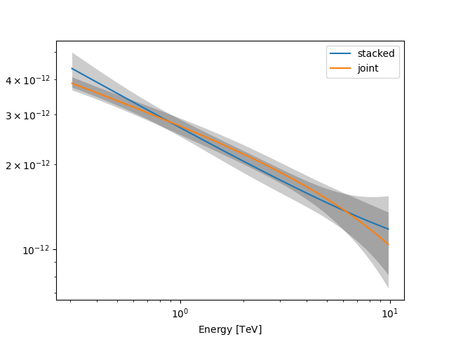
Finally, let us compare the spectral results from the stacked and joint fit:
def plot_spectrum(model, ax, label, color):
    spec = model.spectral_model
    energy_bounds = [0.3, 10] * u.TeV
    spec.plot(
        ax=ax, energy_bounds=energy_bounds, energy_power=2, label=label, color=color
    )
    spec.plot_error(ax=ax, energy_bounds=energy_bounds, energy_power=2, color=color)


fig, ax = plt.subplots()
plot_spectrum(model, ax=ax, label="stacked", color="tab:blue")
plot_spectrum(model_joint, ax=ax, label="joint", color="tab:orange")
ax.legend()
plt.show()
/home/runner/work/gammapy-docs/gammapy-docs/gammapy/.tox/build_docs/lib/python3.12/site-packages/gammapy/modeling/models/spectral.py:649: UserWarning: This axis already has a converter set and is updating to a potentially incompatible converter
  ax.plot(energy.center, flux.quantity[:, 0, 0], **kwargs)
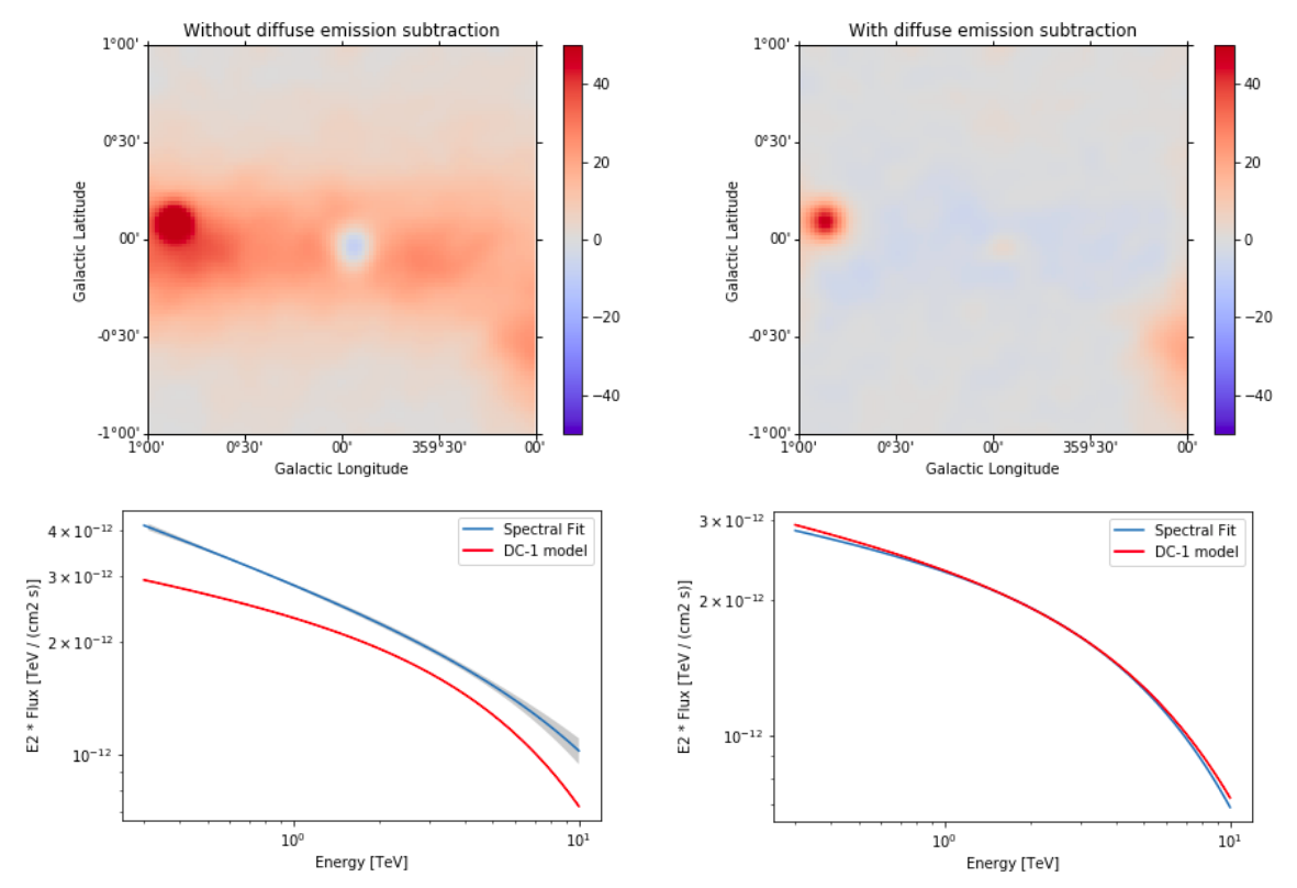
Summary#
Note that this notebook aims to show you the procedure of a 3D analysis using just a few observations. Results get much better for a more complete analysis considering the GPS dataset from the CTA First Data Challenge (DC-1) and also the CTA model for the Galactic diffuse emission, as shown in the next image:
Exercises#
Analyse the second source in the field of view: G0.9+0.1 and add it to the combined model.
Perform modeling in more details.
Add diffuse component, get flux points.
Total running time of the script: (0 minutes 22.969 seconds)