Fermi-LAT with Gammapy

Data inspection and preliminary analysis with Fermi-LAT data.

Introduction

Gammapy fully supports Fermi-LAT data analysis from DL4 level (binned maps). In order to perform data reduction from the events list and spacecraft files to binned counts and IRFs maps we recommend to use Fermipy, which is based on the Fermi Science Tools (Fermi ST).

Using Gammapy with Fermi-LAT data could be an option for you if you want to do an analysis that is not easily possible with Fermipy and the Fermi Science Tools. For example a joint likelihood fit of Fermi-LAT data with data e.g. from H.E.S.S., MAGIC, VERITAS or some other instrument, or analysis of Fermi-LAT data with a complex spatial or spectral model that is not available in Fermipy or the Fermi ST.

This tutorial will show you how to convert Fermi-LAT data into a DL4 format that can be used by Gammapy (MapDataset) and perform a 3D analysis. As an example, we will look at the Galactic center. We are going to analyses high-energy data from 10 GeV from 1 TeV (in reconstructed energy).

Setup

For this notebook you have to get the prepared fermi-gc data provided in your $GAMMAPY_DATA.

# %matplotlib inline

import numpy as np
from astropy import units as u
import matplotlib.pyplot as plt

from gammapy.catalog import CATALOG_REGISTRY
from gammapy.datasets import Datasets, FermipyDatasetsReader
from gammapy.estimators import TSMapEstimator
from gammapy.maps import Map
from gammapy.modeling import Fit
from gammapy.modeling.models import (
    Models,
    PointSpatialModel,
    PowerLawSpectralModel,
    TemplateSpatialModel,
    SkyModel,
    PowerLawNormSpectralModel,
)
from gammapy.utils.scripts import make_path

Check setup

We check the setup in this tutorial, as we require specific files to be downloaded to continue.

from gammapy.utils.check import check_tutorials_setup

check_tutorials_setup()

System:

        python_executable      : /home/runner/work/gammapy-docs/gammapy-docs/gammapy/.tox/build_docs/bin/python
        python_version         : 3.11.13
        machine                : x86_64
        system                 : Linux


Gammapy package:

        version                : 2.0.dev2342+g5815e249e
        path                   : /home/runner/work/gammapy-docs/gammapy-docs/gammapy/.tox/build_docs/lib/python3.11/site-packages/gammapy


Other packages:

        numpy                  : 2.3.3
        scipy                  : 1.16.2
        astropy                : 7.1.1
        regions                : 0.10
        click                  : 8.2.1
        yaml                   : 6.0.3
        IPython                : 9.6.0
        jupyterlab             : not installed
        matplotlib             : 3.9.4
        pandas                 : not installed
        healpy                 : 1.18.1
        iminuit                : 2.31.1
        sherpa                 : 4.18.0
        naima                  : 0.10.2
        emcee                  : 3.1.6
        corner                 : 2.2.3
        ray                    : 2.50.0


Gammapy environment variables:

        GAMMAPY_DATA           : /home/runner/work/gammapy-docs/gammapy-docs/gammapy-datasets/dev

Fermipy configuration file

Gammapy can utilise the same configuration file as Fermipy to convert the Fermipy-generated maps into Gammapy datasets. For more information on the structure of these files, refer to the Fermipy configuration page. In this tutorial, we will analyse Galactic center data generated with Fermipy version 1.3 and the configuration given in $GAMMAPY_DATA/fermi-gc/config_fermipy_gc_example.yaml:

# Fermipy example configuration
# for details, see https://fermipy.readthedocs.io/en/latest/config.html
# For IRFs, event type and event class options, see https://fermi.gsfc.nasa.gov/ssc/data/analysis/documentation/Cicerone/Cicerone_Data/LAT_DP.html
components:
  - model: {isodiff: $FERMI_DIR/refdata/fermi/galdiffuse/iso_P8R3_CLEAN_V3_PSF2_v1.txt}
    selection: {evtype: 16}  #4 is PSF0, 8 PSF1, 16 PSF2, 32 PSF3
    data: {ltcube: null}
  - model: {isodiff: $FERMI_DIR/refdata/fermi/galdiffuse/iso_P8R3_CLEAN_V3_PSF3_v1.txt}
    selection: {evtype: 32}
    data: {ltcube: null}

data:
  evfile : ./raw/events_list.lst
  scfile : ./raw/L241227031840F357373F12_SC00.fits

binning:
  roiwidth   : 8.0
  binsz      : 0.1
  binsperdec   : 10
  coordsys : GAL
  proj: CAR
  projtype: WCS

selection :
# gtselect parameters
  emin : 3981.0717055349733 # ENERGY TRUE for Gammapy
  emax : 2511886.4315095823 # ENERGY TRUE for Gammapy
  zmax    : 105 # deg
  evclass : 256 # CLEAN
  tmin    : 239557417
  tmax    : 752112005

# gtmktime parameters
  filter : 'DATA_QUAL>0 && LAT_CONFIG==1'
  roicut : 'no'

# Set the ROI center to the coordinates of this source
  glon : 0.
  glat : 0.

fileio:
   outdir : ''
   logfile : 'out.log'
   usescratch : False
   scratchdir  : '/scratch'

gtlike:
  edisp : True
  edisp_bins : 0 # DO NOT CHANGE edisp_bins will be handled by Gammapy
  irfs : 'P8R3_CLEAN_V3'

model:
  src_roiwidth : 10.0 # This is used by Fermipy to compute the PSF RADMAX, even if no models are set

The most important points for Gammapy users are:

• emin and emax in this file should be considered as the energy true range. It should be larger that the reconstructed energy range.

• edisp_bins : 0 is strongly recommended at this stage otherwise you might face inconsistencies in the energy axes of the different IRFs created by Fermipy.

• The edisp_bins value will be redefined later on by Gammapy as a positive value in order to create the reconstructed energy axis properly.

• If you want to use the $FERMI_DIR variable to read the background models it must also be defined in your Gammapy environment, otherwise you have to define your own paths.

• For this tutorial we copied the iso files in $GAMMAPY_DATA/fermi-gc and edited the paths in the yaml file for simplicity.

More generally in order to select a good binning it is important to know the instrument resolution, for that you can have a quick look at the IRFs in the Fermi-LAT performance page.

Since the energy resolution varies with energy, it is important to choose an energy binning that is fine enough to capture this energy dependence. That is why we recommend a binning with 8 to 10 bins per decade. The energy axes will be created such as it is linear in log space so it’s better to define emin and emax such as they align with a log binning. Here we have as true energy range \(\log(emin) = 0.6 \sim 4\) GeV to \(\log(emax) = 3.4 \sim 2500\) GeV. While the reconstructed energy range of our analysis will be 10 GeV to 1000 GeV.

The spatial binning should be of the same order of the PSF 68% containment radius which is in average 0.1 degree above 10 GeV and rapidly increases at lower energy. Ideally it should remain within a factor of 2 or 3 of the PSF radius at most. In order to properly take into account for the sources outside the region of interest that contribute inside due to the PSF we have to define a wider roiwidth than our actual region of interest. Typically, we need a margin equal to the 99% containment of the PSF on each side. Above 10 GeV considering only PSF2&3 the 99% PSF containment radius is about 1 degree. Thus, if we want to study a 3 degree radius around the GC we have to take a roiwidth of 8 deg. (If considering lower energies or including PSF0 and PSF1, it should be much larger).

From Fermipy maps to Gammapy datasets

In your Fermipy environment you have to run the following commands

from fermipy.gtanalysis import GTAnalysis
gta = GTAnalysis('config_fermipy_gc_example.yaml',logging={'verbosity' : 3})
gta.setup()

gta.compute_psf(overwrite=True) # this creates the psf kernel
gta.compute_drm(edisp_bins=0, overwrite=True) # this creates the energy dispersion matrix
# DO NOT CHANGE edisp_bins here, it will be redefined by Gammapy later on

This will produce a number of files including:

• “ccube_00.fits” (counts)

• “bexpmap_00.fits” (exposure)

• “psf_00.fits” (psf)

• “drm_00.fits” (edisp)

In your Gammapy environment you can create the datasets using the same configuration file.

reader = FermipyDatasetsReader(
    "$GAMMAPY_DATA/fermi-gc/config_fermipy_gc_example.yaml", edisp_bins=4
)
datasets = reader.read()
print(datasets)

/home/runner/work/gammapy-docs/gammapy-docs/gammapy/.tox/build_docs/lib/python3.11/site-packages/astropy/wcs/wcs.py:806: FITSFixedWarning: 'datfix' made the change 'Set DATEREF to '2001-01-01T00:01:04.184' from MJDREF.
Set MJD-OBS to 54682.655283 from DATE-OBS.
Set MJD-END to 60614.993543 from DATE-END'.
  warnings.warn(
/home/runner/work/gammapy-docs/gammapy-docs/gammapy/.tox/build_docs/lib/python3.11/site-packages/astropy/wcs/wcs.py:806: FITSFixedWarning: 'datfix' made the change 'Set DATEREF to '2001-01-01T00:01:04.184' from MJDREF.
Set MJD-OBS to 54682.655283 from DATE-OBS.
Set MJD-END to 60614.993543 from DATE-END'.
  warnings.warn(
Datasets
--------

Dataset 0:

  Type       : MapDataset
  Name       : P8R3_CLEAN_V3_PSF2_v1
  Instrument :
  Models     : ['isotropic_P8R3_CLEAN_V3_PSF2_v1']

Dataset 1:

  Type       : MapDataset
  Name       : P8R3_CLEAN_V3_PSF3_v1
  Instrument :
  Models     : ['isotropic_P8R3_CLEAN_V3_PSF3_v1']

Note that the edisp_bins is set again here as a positive number so Gammapy can create its reconstructed energy axis properly. The energy dispersion correction implemented Gammapy is closer to the version implemented in Fermitools >1.2.0, which take into account the interplay between the energy dispersion and PSF.

Across most of the Fermi energy range, the level of migration in log10(E) remains within 0.2, increasing up to 0.4 below 100 MeV, due to energy dispersion. Therefore, we recommend that the product of |edisp_bins| and the width of the log10(E) bins be at least equal to 0.2. For a binning of 8 to 10 bins per decade, this corresponds to |edisp_bins| ≥ 2. For further information, see Pass8_edisp_usage. In our case, we have 10 bins per decade and true energy axis starts at about 4 GeV, so with edisp_bins=4 the reconstructed energy axis starts at 10 GeV:

print(datasets[0].exposure.geom.axes["energy_true"])
print(datasets[0].counts.geom.axes["energy"])

MapAxis

        name       : energy_true
        unit       : 'MeV'
        nbins      : 28
        node type  : edges
        edges min  : 4.0e+03 MeV
        edges max  : 2.5e+06 MeV
        interp     : log

MapAxis

        name       : energy
        unit       : 'MeV'
        nbins      : 20
        node type  : edges
        edges min  : 1.0e+04 MeV
        edges max  : 1.0e+06 MeV
        interp     : log

Note that selecting edisp_bins=2 means the reconstructed energy of the counts geometry will start at \(10^{0.8} \sim 6.3\) GeV. If we want to start the analysis at 10 GeV in this case, we need to update the mask_fit to exclude the first 2 reconstructed energy bins. Considering more edisp_bins is generally safer but requires more memory and increases computation time.

Alternatively, if you created the counts and IRF files from the Fermi-LAT science tools without Fermipy you can use the create_dataset method. Note that in this case we cannot guarantee that your maps have the correct axes dimensions to be properly converted into Gammapy datasets.

path = make_path("$GAMMAPY_DATA/fermi-gc")
dataset0 = reader.create_dataset(
    path / "ccube_00.fits",
    path / "bexpmap_00.fits",
    path / "psf_00.fits",
    path / "drm_00.fits",
    isotropic_file=None,
    edisp_bins=0,
    name="fermi_lat_gc_psf2",
)
dataset1 = reader.create_dataset(
    path / "ccube_01.fits",
    path / "bexpmap_01.fits",
    path / "psf_01.fits",
    path / "drm_01.fits",
    isotropic_file=None,
    edisp_bins=0,
    name="fermi_lat_gc_psf3",
)

datasets_fromST = Datasets([dataset0, dataset1])


# The above was an alternative reading method we don't need those after
del dataset0, dataset1, datasets_fromST

/home/runner/work/gammapy-docs/gammapy-docs/gammapy/.tox/build_docs/lib/python3.11/site-packages/astropy/wcs/wcs.py:806: FITSFixedWarning: 'datfix' made the change 'Set DATEREF to '2001-01-01T00:01:04.184' from MJDREF.
Set MJD-OBS to 54682.655283 from DATE-OBS.
Set MJD-END to 60614.993543 from DATE-END'.
  warnings.warn(
/home/runner/work/gammapy-docs/gammapy-docs/gammapy/.tox/build_docs/lib/python3.11/site-packages/astropy/wcs/wcs.py:806: FITSFixedWarning: 'datfix' made the change 'Set DATEREF to '2001-01-01T00:01:04.184' from MJDREF.
Set MJD-OBS to 54682.655283 from DATE-OBS.
Set MJD-END to 60614.993543 from DATE-END'.
  warnings.warn(

Fermi-LAT IRF properties

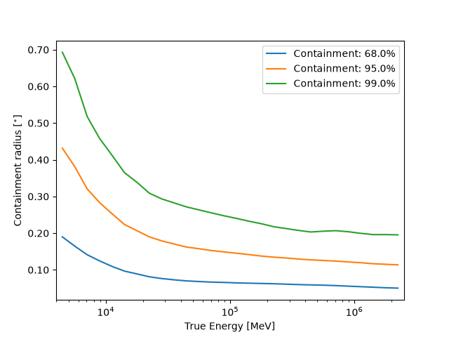
Exposure

Exposure is almost constant across the field of view, with less than 5% variation at a given energy.

datasets[0].exposure.plot_interactive(add_cbar=True)
plt.show()

interactive(children=(SelectionSlider(continuous_update=False, description='Select energy_true:', layout=Layout(width='50%'), options=('3.98 GeV - 5.01 GeV', '5.01 GeV - 6.31 GeV', '6.31 GeV - 7.94 GeV', '7.94 GeV - 10.0 GeV', '10.0 GeV - 12.6 GeV', '12.6 GeV - 15.8 GeV', '15.8 GeV - 20.0 GeV', '20.0 GeV - 25.1 GeV', '25.1 GeV - 31.6 GeV', '31.6 GeV - 39.8 GeV', '39.8 GeV - 50.1 GeV', '50.1 GeV - 63.1 GeV', '63.1 GeV - 79.4 GeV', '79.4 GeV - 100 GeV', '100 GeV - 126 GeV', '126 GeV - 158 GeV', '158 GeV - 200 GeV', '200 GeV - 251 GeV', '251 GeV - 316 GeV', '316 GeV - 398 GeV', '398 GeV - 501 GeV', '501 GeV - 631 GeV', '631 GeV - 794 GeV', '794 GeV - 1 TeV', '1 TeV - 1.26 TeV', '1.26 TeV - 1.58 TeV', '1.58 TeV - 2.00 TeV', '2.00 TeV - 2.51 TeV'), style=SliderStyle(description_width='initial'), value='3.98 GeV - 5.01 GeV'), RadioButtons(description='Select stretch:', index=1, options=('linear', 'sqrt', 'log'), style=DescriptionStyle(description_width='initial'), value='sqrt'), Output()), _dom_classes=('widget-interact',))

PSF

For Fermi-LAT, the PSF only varies little within a given regions of the sky, especially at high energies like what we have here. So we have only one PSF kernel.

datasets[0].psf.plot_containment_radius_vs_energy(fraction=(0.68, 0.95, 0.99))
plt.show()

Region of interest and mask definition

As mentioned previously, the width of dataset is larger that our actual region of interest in order to properly take into account for the sources outside that contributes inside due to the PSF. So we define the valid RoI for fitting by creating a mask_fit.

margin = (
    2.0 * u.deg
)  # >1 deg should be fine for this dataset we take 2 so the notebook is faster
geom = datasets[0].counts.geom
mask_fit = Map.from_geom(geom, data=True, dtype=bool)
mask_fit = mask_fit.binary_erode(width=margin, kernel="disk")

mask_fit.plot_interactive()
plt.show()

interactive(children=(SelectionSlider(continuous_update=False, description='Select energy:', layout=Layout(width='50%'), options=('10.0 GeV - 12.6 GeV', '12.6 GeV - 15.8 GeV', '15.8 GeV - 20.0 GeV', '20.0 GeV - 25.1 GeV', '25.1 GeV - 31.6 GeV', '31.6 GeV - 39.8 GeV', '39.8 GeV - 50.1 GeV', '50.1 GeV - 63.1 GeV', '63.1 GeV - 79.4 GeV', '79.4 GeV - 100 GeV', '100 GeV - 126 GeV', '126 GeV - 158 GeV', '158 GeV - 200 GeV', '200 GeV - 251 GeV', '251 GeV - 316 GeV', '316 GeV - 398 GeV', '398 GeV - 501 GeV', '501 GeV - 631 GeV', '631 GeV - 794 GeV', '794 GeV - 1 TeV'), style=SliderStyle(description_width='initial'), value='10.0 GeV - 12.6 GeV'), RadioButtons(description='Select stretch:', index=1, options=('linear', 'sqrt', 'log'), style=DescriptionStyle(description_width='initial'), value='sqrt'), Output()), _dom_classes=('widget-interact',))

Now we attach it the datasets

for d in datasets:
    d.mask_fit = mask_fit

Models

Isotropic diffuse background

The FermipyDatasetsReader also created one isotropic diffuse model for each dataset:

models_iso = Models(datasets.models)
print(models_iso)

Models

Component 0: SkyModel

  Name                      : isotropic_P8R3_CLEAN_V3_PSF2_v1
  Datasets names            : ['P8R3_CLEAN_V3_PSF2_v1']
  Spectral model type       : CompoundSpectralModel
  Spatial  model type       : ConstantSpatialModel
  Temporal model type       :
  Parameters:
    tilt                  (frozen):      0.000
    norm                          :      1.000   +/-    0.00
    reference             (frozen):      1.000       TeV
    value                 (frozen):      1.000       1 / sr

Component 1: SkyModel

  Name                      : isotropic_P8R3_CLEAN_V3_PSF3_v1
  Datasets names            : ['P8R3_CLEAN_V3_PSF3_v1']
  Spectral model type       : CompoundSpectralModel
  Spatial  model type       : ConstantSpatialModel
  Temporal model type       :
  Parameters:
    tilt                  (frozen):      0.000
    norm                          :      1.000   +/-    0.00
    reference             (frozen):      1.000       TeV
    value                 (frozen):      1.000       1 / sr

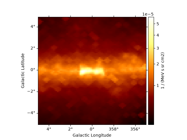
Galactic diffuse background

The Fermi-LAT collaboration provides a galactic diffuse emission model, that can be used as a background model for Fermi-LAT source analysis. These files are called usually IEM for interstellar emission model, the latest is gll_iem_v07.fits. For details see the BackgroundModels page. If you have Fermipy installed it can also be found in $FERMI_DIR/refdata/fermi/galdiffuse/gll_iem_v07.fits

Diffuse model maps are very large (100s of MB), so as an example here, we just load one that represents a small cutout for the Galactic center region.

In this case, the maps are already in differential units, so we do not want to normalise it again.

template_iem = TemplateSpatialModel.read(
    filename="$GAMMAPY_DATA/fermi-gc/gll_iem_v07_gc.fits.gz", normalize=False
)

model_iem = SkyModel(
    spectral_model=PowerLawNormSpectralModel(),
    spatial_model=template_iem,
    name="diffuse-iem",
)

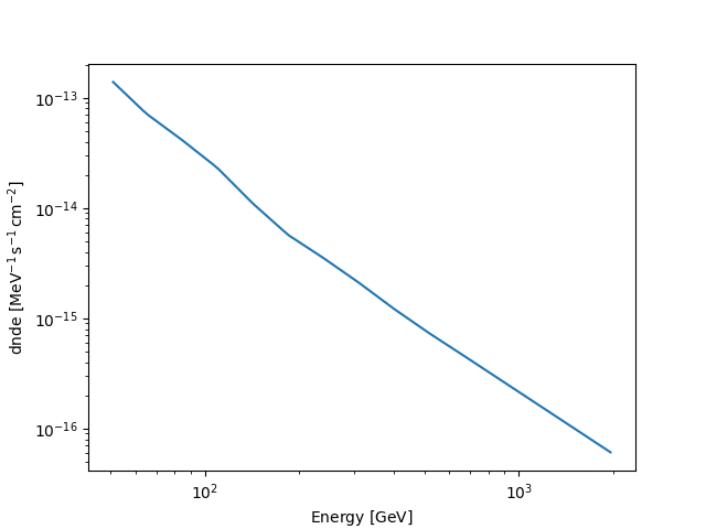
Let’s look at the template :

template_iem.map.plot_interactive(add_cbar=True)
plt.show()


models_diffuse = models_iso + model_iem

interactive(children=(SelectionSlider(continuous_update=False, description='Select energy_true:', layout=Layout(width='50%'), options=('50.0 MeV', '65.0 MeV', '84.5 MeV', '110 MeV', '143 MeV', '185 MeV', '241 MeV', '313 MeV', '407 MeV', '529 MeV', '687 MeV', '893 MeV', '1.16 GeV', '1.51 GeV', '1.96 GeV', '2.55 GeV', '3.31 GeV', '4.31 GeV', '7.27 GeV', '12.3 GeV', '20.8 GeV', '35.0 GeV', '59.2 GeV', '100.0 GeV', '169 GeV', '285 GeV', '482 GeV', '814 GeV'), style=SliderStyle(description_width='initial'), value='50.0 MeV'), RadioButtons(description='Select stretch:', index=1, options=('linear', 'sqrt', 'log'), style=DescriptionStyle(description_width='initial'), value='sqrt'), Output()), _dom_classes=('widget-interact',))

Sources

Source models can be loaded from the 4FGL catalog directly available in $GAMMAPY_DATA. For details see the Fermi-LAT catalog page.

catalog_4fgl = CATALOG_REGISTRY.get_cls("4fgl")()  # load 4FGL catalog

We want to select only the sources inside the dataset spatial geometry:

in_geom = geom.to_image().contains(catalog_4fgl.positions)
catalog_4fgl_gc = catalog_4fgl[in_geom]

models_4fgl_gc = catalog_4fgl_gc.to_models()

/home/runner/work/gammapy-docs/gammapy-docs/gammapy/.tox/build_docs/lib/python3.11/site-packages/gammapy/catalog/fermi.py:587: UserWarning: Warning: converting a masked element to nan.
  "index_2": np.nan_to_num(float(self.data["Unc_PLEC_Exp_Index"])),
/home/runner/work/gammapy-docs/gammapy-docs/gammapy/.tox/build_docs/lib/python3.11/site-packages/gammapy/catalog/fermi.py:587: UserWarning: Warning: converting a masked element to nan.
  "index_2": np.nan_to_num(float(self.data["Unc_PLEC_Exp_Index"])),
/home/runner/work/gammapy-docs/gammapy-docs/gammapy/.tox/build_docs/lib/python3.11/site-packages/gammapy/catalog/fermi.py:587: UserWarning: Warning: converting a masked element to nan.
  "index_2": np.nan_to_num(float(self.data["Unc_PLEC_Exp_Index"])),

That’s still quite a lot of sources

print("Number of source models", len(models_4fgl_gc))

Number of source models 110

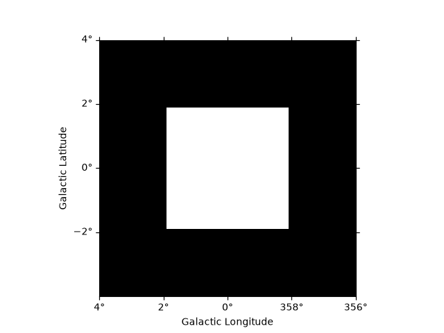
In order to improve performances we can store all the sources outside the mask_fit region into a single template (the same could be done for all the sources we want to keep frozen).

sources_ouside_roi = models_4fgl_gc.select_mask(~mask_fit, use_evaluation_region=False)
sources_inside_roi = Models([m for m in models_4fgl_gc if m not in sources_ouside_roi])

geom_true = datasets[0].exposure.geom
sources_outside_roi = sources_ouside_roi.to_template_sky_model(
    geom_true, name="sources_outside"
)

sources_outside_roi.spatial_model.filename = "sources_outside.fits"

sources_outside_roi.spatial_model.map.plot_interactive(add_cbar=True)
plt.show()

interactive(children=(SelectionSlider(continuous_update=False, description='Select energy_true:', layout=Layout(width='50%'), options=('3.98 GeV - 5.01 GeV', '5.01 GeV - 6.31 GeV', '6.31 GeV - 7.94 GeV', '7.94 GeV - 10.0 GeV', '10.0 GeV - 12.6 GeV', '12.6 GeV - 15.8 GeV', '15.8 GeV - 20.0 GeV', '20.0 GeV - 25.1 GeV', '25.1 GeV - 31.6 GeV', '31.6 GeV - 39.8 GeV', '39.8 GeV - 50.1 GeV', '50.1 GeV - 63.1 GeV', '63.1 GeV - 79.4 GeV', '79.4 GeV - 100 GeV', '100 GeV - 126 GeV', '126 GeV - 158 GeV', '158 GeV - 200 GeV', '200 GeV - 251 GeV', '251 GeV - 316 GeV', '316 GeV - 398 GeV', '398 GeV - 501 GeV', '501 GeV - 631 GeV', '631 GeV - 794 GeV', '794 GeV - 1 TeV', '1 TeV - 1.26 TeV', '1.26 TeV - 1.58 TeV', '1.58 TeV - 2.00 TeV', '2.00 TeV - 2.51 TeV'), style=SliderStyle(description_width='initial'), value='3.98 GeV - 5.01 GeV'), RadioButtons(description='Select stretch:', index=1, options=('linear', 'sqrt', 'log'), style=DescriptionStyle(description_width='initial'), value='sqrt'), Output()), _dom_classes=('widget-interact',))

Now we have less models to describe the sources

models_sources = sources_inside_roi + sources_outside_roi

print("Number of source models", len(models_sources))

Number of source models 28

Fit

Now, the big finale: let’s do a 3D of the brightest sources and IEM models.

First we attach the models to the datasets.

models = models_sources + models_diffuse

datasets.models = models

print("Number of models", len(models))

Number of models 31

Let’s find the 3 brightest sources:

n_brightest = 3
integrated_flux = u.Quantity(
    [m.spectral_model.integral(10 * u.GeV, 1 * u.TeV) for m in sources_inside_roi]
)
order = np.argsort(integrated_flux)
selected_sources = Models([sources_inside_roi[int(ii)] for ii in order[:n_brightest]])

print(selected_sources.names)

free_models = selected_sources + model_iem

['4FGL J1739.4-3015', '4FGL J1751.6-3002', '4FGL J1754.3-2915']

We keep only their normalisation free for simplicity:

models.freeze()  # freeze all parameters

# and unfreeze only the amplitude or norm of the selected models
for p in free_models.parameters:
    if p.name in ["amplitude", "norm"]:
        p.frozen = False
        p.min = 0

print("Number of free parameters", len(models.parameters.free_parameters))

fit = Fit()
result = fit.run(datasets=datasets)

print(result)

Number of free parameters 4
OptimizeResult

        backend    : minuit
        method     : migrad
        success    : True
        message    : Optimization terminated successfully.
        nfev       : 97
        total stat : 20322.54

CovarianceResult

        backend    : minuit
        method     : hesse
        success    : True
        message    : Hesse terminated successfully.

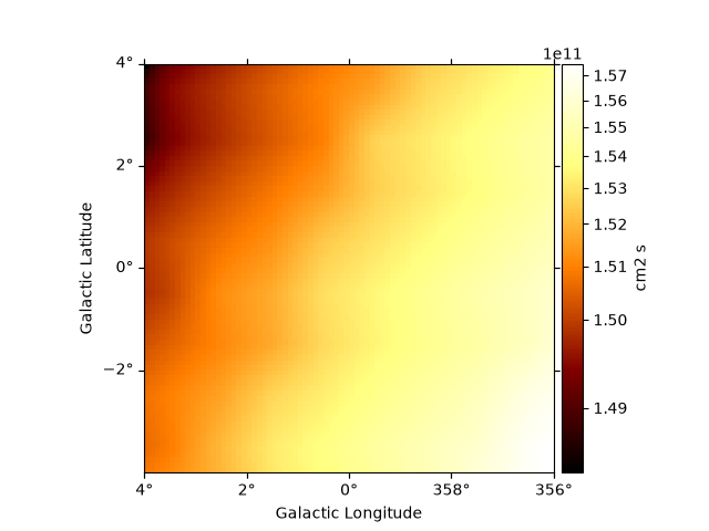
Residual TS map

Now we can look at the residual TS map to check there is no significant excess left:

spatial_model = PointSpatialModel()
spectral_model = PowerLawSpectralModel(index=2)
model = SkyModel(spatial_model=spatial_model, spectral_model=spectral_model)

ts_estimator = TSMapEstimator(
    model,
    kernel_width="1 deg",  # this set close to the 95-99% containment radius of the PSF
    selection_optional=[],
    sum_over_energy_groups=True,
    energy_edges=[10, 1000] * u.GeV,
)


ts_results = ts_estimator.run(datasets)


image = ts_results["sqrt_ts"]
image = image.cutout(
    image.geom.center_skydir, width=np.max(image.geom.width) - 2 * margin
)

fig = plt.figure(figsize=(7, 5))
ax = image.plot(
    clim=[-8, 8],
    cmap=plt.cm.RdBu_r,
    add_cbar=True,
    kwargs_colorbar={"label": r"$\sqrt{TS}$ [$\sigma$]"},
)
sources_inside_roi.plot_regions(
    ax=ax, edgecolor="g", linestyle="-", kwargs_point=dict(marker=".")
)
plt.show()

Serialisation

To serialise the created dataset, you must proceed through the Datasets API

datasets.write(
    filename="fermi_lat_gc_datasets.yaml",
    filename_models="fermi_lat_gc_models.yaml",
    overwrite=True,
)
datasets_read = Datasets.read(
    filename="fermi_lat_gc_datasets.yaml", filename_models="fermi_lat_gc_models.yaml"
)

Exercises

• Fit the position and spectrum of the source SNR G0.9+0.1.

• Make maps and fit the position and spectrum of the Crab nebula.

Summary

In this tutorial you have seen how to work with Fermi-LAT data with Gammapy. You have to use Fermipy or the Fermi ST to perform the data reduction then you can use Gammapy for analysis using the same methods that are used to analyse IACT data.