This is a fixed-text formatted version of a Jupyter notebook

• Try online

• You can contribute with your own notebooks in this GitHub repository.

• Source files: image_analysis.ipynb | image_analysis.py

Fitting 2D images with Gammapy

Gammapy does not have any special handling for 2D images, but treats them as a subset of maps. Thus, classical 2D image analysis can be done in 2 independent ways:

1. Using the sherpa package

2. Within gammapy, by assuming 2D analysis to be a sub-set of the generalised maps. Thus, analysis should proceed exactly as demonstrated in analysis_3d.ipynb, taking care of a few things that we mention in this tutorial

We consider 2D images to be a special case of 3D maps, ie, maps with only one energy bin. This is a major difference while analysing in sherpa, where the maps must not contain any energy axis. In this tutorial, we do a classical image analysis using three example observations of the Galactic center region with CTA - i.e., study the source flux and morphology.

Setup

%matplotlib inline
import matplotlib.pyplot as plt
import numpy as np
from scipy.stats import norm

import astropy.units as u
from astropy.coordinates import SkyCoord
from astropy.convolution import Tophat2DKernel
from regions import CircleSkyRegion

from gammapy.detect import compute_lima_on_off_image
from gammapy.data import DataStore
from gammapy.irf import make_mean_psf
from gammapy.maps import Map, MapAxis, WcsGeom
from gammapy.cube import (
    SafeMaskMaker,
    PSFKernel,
    MapDataset,
    MapDatasetMaker,
    MapDatasetOnOff,
    RingBackgroundMaker,
)
from gammapy.modeling.models import (
    SkyModel,
    BackgroundModel,
    PowerLaw2SpectralModel,
    PointSpatialModel,
)
from gammapy.modeling import Fit

Prepare modeling input data

The counts, exposure and the background maps

This is the same drill - use DataStore object to access the CTA observations and retrieve a list of observations by passing the observations IDs to the .get_observations() method, then use MapMaker to make the maps.

# Define which data to use and print some information
data_store = DataStore.from_dir("$GAMMAPY_DATA/cta-1dc/index/gps/")
data_store.info()

Data store:
HDU index table:
BASE_DIR: /Users/adonath/data/gammapy-data/cta-1dc/index/gps
Rows: 24
OBS_ID: 110380 -- 111630
HDU_TYPE: ['aeff', 'bkg', 'edisp', 'events', 'gti', 'psf']
HDU_CLASS: ['aeff_2d', 'bkg_3d', 'edisp_2d', 'events', 'gti', 'psf_3gauss']


Observation table:
Observatory name: 'N/A'
Number of observations: 4

data_store.obs_table["ONTIME"].quantity.sum().to("hour")

$$2 \; \mathrm{h}$$

# Select some observations from these dataset by hand
obs_ids = [110380, 111140, 111159]
observations = data_store.get_observations(obs_ids)

emin, emax = [0.1, 10] * u.TeV
energy_axis = MapAxis.from_bounds(
    emin.value, emax.value, 10, unit="TeV", name="energy", interp="log"
)
geom = WcsGeom.create(
    skydir=(0, 0),
    binsz=0.02,
    width=(10, 8),
    coordsys="GAL",
    proj="CAR",
    axes=[energy_axis],
)

Note that even when doing a 2D analysis, it is better to use fine energy bins in the beginning and then sum them over. This is to ensure that the background shape can be approximated by a power law function in each energy bin. The run_images() can be used to compute maps in fine bins and then squash them to have one bin. This can be done by specifying keep_dims = True. This will compute a summed counts and background maps, and a spectral weighted exposure map.

stacked = MapDataset.create(geom)

%%time
maker = MapDatasetMaker(selection=["counts", "exposure", "background"])
maker_safe_mask = SafeMaskMaker(methods=["offset-max"], offset_max=4.0 * u.deg)

datasets = []

for obs in observations:
    cutout = stacked.cutout(obs.pointing_radec, width="8 deg")
    dataset = maker.run(cutout, obs)
    dataset = maker_safe_mask.run(dataset, obs)
    datasets.append(dataset)
    stacked.stack(dataset)

CPU times: user 3.59 s, sys: 934 ms, total: 4.53 s
Wall time: 4.75 s

spectrum = PowerLaw2SpectralModel(index=2)
dataset_2d = stacked.to_image(spectrum=spectrum)

maps2D = {
    "counts": dataset_2d.counts,
    "exposure": dataset_2d.exposure,
    "background": dataset_2d.background_model.map,
}

For a typical 2D analysis, using an energy dispersion usually does not make sense. A PSF map can be made as in the regular 3D case, taking care to weight it properly with the spectrum.

# mean PSF
geom2d = maps2D["exposure"].geom
src_pos = SkyCoord(0, 0, unit="deg", frame="galactic")
table_psf = make_mean_psf(observations, src_pos)

table_psf_2d = table_psf.table_psf_in_energy_band(
    (emin, emax), spectrum=spectrum
)

# PSF kernel used for the model convolution
psf_kernel = PSFKernel.from_table_psf(
    table_psf_2d, geom2d, max_radius="0.3 deg"
)

Now, the analysis proceeds as usual. Just take care to use the proper geometry in this case.

Define a mask

region = CircleSkyRegion(center=src_pos, radius=0.6 * u.deg)
mask = Map.from_geom(geom2d, data=geom2d.region_mask([region]))

Modeling the source

This is the important thing to note in this analysis. Since modeling and fitting in gammapy.maps needs to have a combination of spectral models, we have to use a dummy Powerlaw as for the spectral model and fix its index to 2. Since we are interested only in the integral flux, we will use the PowerLaw2SpectralModel model which directly fits an integral flux.

spatial_model = PointSpatialModel(
    lon_0="0.01 deg", lat_0="0.01 deg", frame="galactic"
)
spectral_model = PowerLaw2SpectralModel(
    emin=emin, emax=emax, index=2.0, amplitude="3e-12 cm-2 s-1"
)
model = SkyModel(spatial_model=spatial_model, spectral_model=spectral_model)
model.parameters["index"].frozen = True

Modeling the background

Gammapy fitting framework assumes the background to be an integrated model. Thus, we will define the background as a model, and freeze its parameters for now.

background_model = BackgroundModel(maps2D["background"])
background_model.parameters["norm"].frozen = True
background_model.parameters["tilt"].frozen = True

dataset = MapDataset(
    models=model,
    counts=maps2D["counts"],
    exposure=maps2D["exposure"],
    background_model=background_model,
    mask_fit=mask,
    psf=psf_kernel,
)

%%time
fit = Fit([dataset])
result = fit.run()

CPU times: user 1.02 s, sys: 15 ms, total: 1.04 s
Wall time: 1.04 s

To see the actual best-fit parameters, do a print on the result

print(model)

SkyModel

   name     value    error   unit      min        max    frozen
--------- ---------- ----- -------- ---------- --------- ------
    lon_0 -5.363e-02   nan      deg        nan       nan  False
    lat_0 -5.057e-02   nan      deg -9.000e+01 9.000e+01  False
amplitude  4.294e-11   nan cm-2 s-1        nan       nan  False
    index  2.000e+00   nan                 nan       nan   True
     emin  1.000e-01   nan      TeV        nan       nan   True
     emax  1.000e+01   nan      TeV        nan       nan   True

result.parameters.to_table()

Table length=9

name	value	error	unit	min	max	frozen
str9	float64	float64	str8	float64	float64	bool
lon_0	-5.363e-02	3.261e-03	deg	nan	nan	False
lat_0	-5.057e-02	3.308e-03	deg	-9.000e+01	9.000e+01	False
amplitude	4.294e-11	1.747e-12	cm-2 s-1	nan	nan	False
index	2.000e+00	0.000e+00		nan	nan	True
emin	1.000e-01	0.000e+00	TeV	nan	nan	True
emax	1.000e+01	0.000e+00	TeV	nan	nan	True
norm	1.000e+00	0.000e+00		0.000e+00	nan	True
tilt	0.000e+00	0.000e+00		nan	nan	True
reference	1.000e+00	0.000e+00	TeV	nan	nan	True

result.parameters.correlation[:4, :4]

/Users/adonath/github/adonath/gammapy/gammapy/modeling/parameter.py:528: RuntimeWarning: invalid value encountered in true_divide
  return self.covariance / np.outer(err, err)

array([[ 1.        ,  0.07391212, -0.02417381,         nan],
       [ 0.07391212,  1.        , -0.03242375,         nan],
       [-0.02417381, -0.03242375,  1.        ,         nan],
       [        nan,         nan,         nan,         nan]])

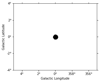
Classical Ring Background Analysis

No we repeat the same analysis but using a classical ring background estimation. We define an exclusion mask and then use the gammapy.cube.RingBackgroundMaker.

geom_image = geom.to_image().to_cube([energy_axis.squash()])

regions = CircleSkyRegion(center=spatial_model.position, radius=0.3 * u.deg)

exclusion_mask = Map.from_geom(geom_image)
exclusion_mask.data = geom_image.region_mask([regions], inside=False)
exclusion_mask.sum_over_axes().plot();

ring_maker = RingBackgroundMaker(
    r_in="0.3 deg", width="0.3 deg", exclusion_mask=exclusion_mask
)

%%time
stacked_on_off = MapDatasetOnOff.create(geom=geom_image)

for dataset in datasets:
    dataset_image = dataset.to_image()
    dataset_on_off = ring_maker.run(dataset_image)
    stacked_on_off.stack(dataset_on_off)

/Users/adonath/software/anaconda3/envs/gammapy-dev/lib/python3.7/site-packages/astropy/units/quantity.py:464: RuntimeWarning: invalid value encountered in true_divide
  result = super().__array_ufunc__(function, method, *arrays, **kwargs)

CPU times: user 290 ms, sys: 100 ms, total: 390 ms
Wall time: 396 ms

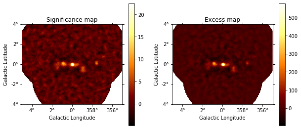
Based on the estimate of the ring background we compute a Li&Ma significance image:

scale = geom.pixel_scales[0].to("deg")
# Using a convolution radius of 0.05 degrees
theta = 0.15 * u.deg / scale
tophat = Tophat2DKernel(theta)
tophat.normalize("peak")

lima_maps = compute_lima_on_off_image(
    stacked_on_off.counts,
    stacked_on_off.counts_off,
    stacked_on_off.acceptance,
    stacked_on_off.acceptance_off,
    tophat,
)

significance_map = lima_maps["significance"]
excess_map = lima_maps["excess"]

That is what the excess and significance look like:

plt.figure(figsize=(10, 10))
ax1 = plt.subplot(221, projection=significance_map.geom.wcs)
ax2 = plt.subplot(222, projection=excess_map.geom.wcs)

ax1.set_title("Significance map")
significance_map.get_image_by_idx((0,)).plot(ax=ax1, add_cbar=True)

ax2.set_title("Excess map")
excess_map.get_image_by_idx((0,)).plot(ax=ax2, add_cbar=True)

(<Figure size 720x720 with 4 Axes>,
 <matplotlib.axes._subplots.WCSAxesSubplot at 0x11f23dd30>,
 <matplotlib.colorbar.Colorbar at 0x123282a90>)

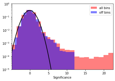
Finally we take a look at the signficance distribution outside the exclusion region:

# create a 2D mask for the images
significance_map_off = significance_map * exclusion_mask

significance_all = significance_map.data[np.isfinite(significance_map.data)]
significance_off = significance_map_off.data[
    np.isfinite(significance_map_off.data)
]

plt.hist(
    significance_all,
    density=True,
    alpha=0.5,
    color="red",
    label="all bins",
    bins=21,
)

plt.hist(
    significance_off,
    density=True,
    alpha=0.5,
    color="blue",
    label="off bins",
    bins=21,
)

# Now, fit the off distribution with a Gaussian
mu, std = norm.fit(significance_off)
x = np.linspace(-8, 8, 50)
p = norm.pdf(x, mu, std)
plt.plot(x, p, lw=2, color="black")
plt.legend()
plt.xlabel("Significance")
plt.yscale("log")
plt.ylim(1e-5, 1)
xmin, xmax = np.min(significance_all), np.max(significance_all)
plt.xlim(xmin, xmax)

print(f"Fit results: mu = {mu:.2f}, std = {std:.2f}")

Fit results: mu = -0.04, std = 1.27

Exercises

1. Update the exclusion mask in the ring background example by thresholding the significance map and re-run the background estimator

2. Plot residual maps as done in the analysis_3d notebook

3. Iteratively add and fit sources